#Topic
These are the concepts, models, and research resources I find myself looking up while studying computer vision and deep learning. I keep adding to the explanations and equations as I study.
#Selected topics
#Contents
| Topic | Content | Notes | Link |
|---|---|---|---|
| Computer Vision | Computer vision concepts | Foundations | Go to section |
| Transformer | Go to section | ||
| RNN | Go to section | ||
| LSTM | Go to section | ||
| ViT | Go to section | ||
| HR Net | Go to section | ||
| GCN | Go to section |
One piece of advice from my professor was to account for computing resources early. Foundation models and vision transformers can be expensive to run.
#Computer Vision
Computer vision develops methods that let computers interpret images and videos.
#Computer vision websites
- CVonline collects explanations of computer vision topics, including links to Wikipedia, databases, literature, and software.
- VisionBib indexes computer vision publications by subject, author, date, journal, and conference.
- Computer Vision Online covers developments and news in the field.
#Computer vision journals
- International Journal of Computer Vision (IJCV) publishes computer vision research and review papers.
- Image and Vision Computing covers image processing and computer vision.
- Computer Vision and Image Understanding publishes research on vision and image understanding.
- Foundations and Trends in Computer Graphics and Vision covers developments in graphics and vision.
- Pattern Recognition publishes research on pattern recognition.
- IEEE Transactions on Image Processing covers image processing.
- IEEE Transactions on Pattern Analysis and Machine Intelligence (TPAMI) covers pattern analysis and machine learning.
- ACM Transactions on Graphics publishes computer graphics research.
#Conferences
- International Conference on Computer Vision (ICCV) is an international venue for computer vision research and techniques.
- IEEE/CVF Conference on Computer Vision and Pattern Recognition (CVPR) covers vision and pattern recognition.
- European Conference on Computer Vision (ECCV) brings together vision researchers in Europe.
- Asian Conference on Computer Vision (ACCV) brings together vision researchers in Asia.
- British Machine Vision Conference (BMVC) presents machine vision research in the UK.
- International Conference on Pattern Recognition (ICPR) covers advances in pattern recognition.
- The organizer, the International Association for Pattern Recognition (IAPR), brings researchers together to share results and techniques.
- IEEE International Conference on Image Processing (ICIP) covers image processing.
- ACM SIGGRAPH presents advances in computer graphics.
#Transformer
Attention Is All You Need
Softmax converts an input vector into a probability distribution. For component i, it is defined as follows.
#RNN
Recurrent neural network
#Vanishing gradients
Building a deep neural network often means stacking many hidden layers. The number of layers and their widths affect both performance and complexity. Larger networks generally contain more trainable weights and biases.
Weights
- A weight determines how strongly an input contributes to a calculation.
- Each connection multiplies its input by its weight.
Biases
- A bias changes how easily a node becomes active.
- Alongside the weights, it adjusts the node’s output.
Backpropagation
- A loss function measures the error between the output and the target.
- Backpropagation computes how the loss depends on each weight and bias so the optimizer can reduce the error.
Gradient descent
- Gradient descent updates the weights and biases in a direction that reduces the loss.
- The learning rate controls the step size and influences how quickly learning proceeds.
Here is the weight on input , and is the bias.
In a deep network, a gradient can shrink as it propagates through many hidden layers. The slope of the activation function enters at every step of backpropagation.
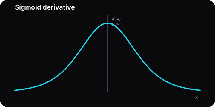
Sigmoid
The sigmoid derivative is positive, approaches zero at the extremes, and reaches a maximum of 0.25, or one quarter, at zero.
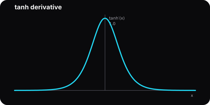
Hyperbolic tangent
The derivative of tanh reaches 1 at zero and approaches zero as the input grows large in magnitude.
#Activation functions
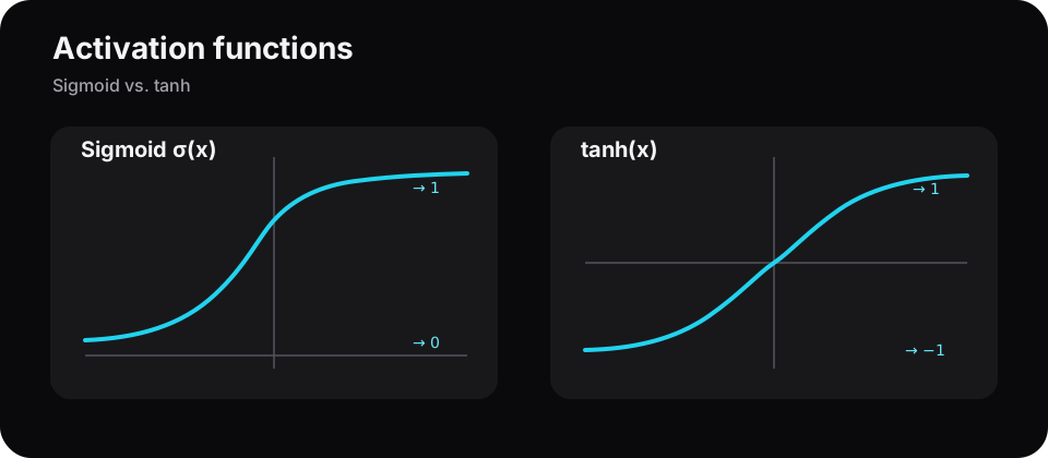
- Sigmoid
- tanh
Both curves illustrate why gradients can vanish when activations saturate.
#MLP
Multilayer perceptron
#Understanding the multilayer perceptron
- The MLP is a foundational machine learning model.
- It is a feedforward neural network with multiple layers.
#Overview
An MLP can learn complex, nonlinear relationships in data. Applications include image recognition, natural language processing, and speech recognition.
#History
The early single-layer perceptron could separate linearly separable data. Real data often have nonlinear boundaries, motivating networks with multiple layers.
Several researchers independently developed ideas behind backpropagation in the early 1970s. Backpropagation became an essential method for training multilayer networks and contributed to the development of deep learning.
#2. MLP architecture: layers and neurons
A typical MLP has an input layer, one or more hidden layers, and an output layer.
The input layer receives raw data, with one input per feature. Hidden layers transform those inputs into new representations. The designer chooses the number of hidden layers and the number of neurons in each as hyperparameters. The output layer produces the prediction. For a multiclass classifier, for example, the number of outputs usually equals the number of classes.1
Each neuron multiplies its inputs from the previous layer by their weights, sums them, adds a bias, and applies an activation function. The weights determine the strengths of the connections. The bias shifts the input to the activation function.1
In a fully connected MLP, every neuron in one layer connects to every neuron in the next.1 These connections support complex patterns, but the number of weights and biases can raise computational cost and the risk of overfitting.3
3. Training an MLP with backpropagation
Supervised learning uses labeled examples to learn a relationship between inputs and outputs.1 During the forward pass, an input moves through the layers to produce a prediction.1 A loss function compares that prediction with its target.8 Common losses include mean squared error for regression and cross-entropy for classification.13
During the backward pass, backpropagation uses the chain rule to compute the gradient of the loss with respect to each weight and bias.2 An optimizer updates the parameters in a direction that reduces the loss.1 The learning rate controls the size of each update.1 Options include gradient descent, stochastic gradient descent (SGD), and Adam.2 Computing all the parameter gradients efficiently makes it practical to train deep MLPs and learn internal features that would otherwise need manual feature engineering.2
4. Activation functions introduce nonlinearity
An activation function acts on each neuron’s weighted sum. Nonlinear activations let an MLP model complex relationships.1 Without them, a stack of affine layers reduces to one affine transformation.2 Common choices include:
- Sigmoid maps values into the interval from 0 to 1. It was common in early hidden layers and is still used in binary classification outputs. ReLU has largely displaced it in hidden layers.2, 13
- tanh maps inputs into the interval from −1 to 1.1
- ReLU (rectified linear unit) passes positive inputs through and returns zero for negative inputs.1 It is inexpensive to compute and helps reduce vanishing gradients, but a unit can become inactive and stop learning, the “dying ReLU” problem.24
- Softmax produces a distribution over classes and is common in multiclass output layers.1
Other choices include Leaky ReLU and Softplus.2 The appropriate function depends on the task and the layer.1 Moving from the Heaviside step function of early perceptrons to activations with useful derivatives, such as sigmoid or the piecewise-linear ReLU, made gradient-based training practical.2
5. Applications
An MLP can support many supervised learning tasks.14 Examples in the source notes include:
- Image recognition and classification. Recognizing objects, digits, and faces in images.1
- Speech recognition. Converting speech data to text.1
- Natural language processing. Modeling meaning for sentiment analysis and machine translation.1
- Time series. Forecasting values such as stock prices or weather from past observations.12
- Regression. Predicting a continuous value.1
- Compression and encryption. Learning data representations for reconstruction or concealment.18
- Autonomous driving. Detecting objects and adjusting a path.18
- Customer relationship management. Profiling and ranking users.18
- Medical diagnosis. Assisting with medical image analysis and disease classification.19
- Recommender systems. Predicting product or content preferences.19
- Financial forecasting. Estimating market trends.24
- Healthcare and biomedicine. Modeling a range of biological and medical problems.24
- Robotics and autonomous systems. Robot control and perception of the environment.24
- Games and reinforcement learning. Making decisions in complex environments.24
- Bioinformatics. Analyzing biological data.28
- Sleep apnea detection. Identifying events from wearable sensor data.28
- Water quality. Predicting water quality parameters.28
- Wind-speed profiles. Estimating profiles from ground observations.28
- Social functioning. Identifying individuals at risk of impaired social function.30
- Driver drowsiness. Detecting drowsiness from EEG signals.10
- Drug development. Applications include drug design and target validation.10
- Urban landscapes. Studying relationships between the built environment and mental state.10
- Pest management. Predicting pest populations to inform control strategies.28
- Career guidance. Generating real-time recommendations from adolescents’ performance in computer games.28
- Orthopedics. Predicting coronal knee alignment after opening-wedge high tibial osteotomy to support surgical planning and analysis.
- Marine energy management. Providing a benchmark for an incremental-learning framework that predicts ship fuel use under changing marine conditions.28
- Electricity demand. Combining MLPs with fuzzy clustering to improve consumption forecasts in regions with changing demand.28
- Medical imaging. Using brain MRI features in a radiomics model to predict the presence and severity of chronic hepatic encephalopathy in adults with cirrhosis.28
- Stock market trends. Comparing an MLP with a Bayesian classifier enhanced by heuristic likelihood estimation.28
- Hydropower runoff. Evaluating MLPs individually and in voting ensembles for daily runoff forecasts in hydropower catchments.28
- Oncology. Comparing MLPs with other models for predicting six-month survival in patients with malignant colorectal cancer to support clinical decisions.28
- Customer demand. Comparing an MLP with an LSTM that incorporates customer behavior to improve demand forecasts.28
- Wind loads. Predicting wind loads on container ships with different container arrangements to support stability, maneuverability, and fuel efficiency.28
- Photovoltaic power. Combining MLPs with models such as the interactive feature trend transformer (IFTformer) for medium- and long-term forecasts.28
- Remaining useful life. Comparing MLPs with models such as CNN-GRU for estimating turbofan engine life in predictive maintenance.28
- Slope stability. Incorporating an MLP into an incremental Bayesian learning model trained on published data for efficient slope stability predictions.28
- Gestational diabetes. Estimating risk early in pregnancy with a neural network and techniques such as NearMiss to identify potential risk factors.28
- Autism spectrum research. Using BrainAGE analysis and individually weighted multilayer perceptron (ILWMLP) regression to identify atypical development in sensorimotor brain networks.28
- Information diffusion. Combining subgraph sampling and multi-head attention to fuse temporal and structural information for prediction in online social networks.28
| Application | Examples |
|---|---|
| Image recognition | Object detection, facial recognition, digit classification |
| Natural language processing | Sentiment analysis, machine translation |
| Time-series forecasting | Stock prices, weather |
| Medical diagnosis | Medical image analysis, disease diagnosis |
| Autonomous driving | Object detection, path adjustment |
6. Strengths and limitations
An MLP can approximate nonlinear functions and learn complex relationships.1 Through its hidden layers it can learn hierarchical features directly from raw inputs.12 MLPs can handle many application areas, with appropriate preprocessing for numerical and categorical features and missing values.12 Hardware and optimization advances make larger datasets and architectures feasible.12 After training, inference can be fast.6 Some tasks yield reasonable accuracy with relatively small datasets, and online learning can update a model incrementally.7
Small datasets and overly complex architectures increase the risk of overfitting.6 Deep models can suffer vanishing or exploding gradients.8 Results are sensitive to hyperparameters such as the learning rate and layer sizes.12 Training a deep MLP can consume substantial computing resources6 and time.25 Its predictions can be difficult to explain.25 Dense connections increase parameter count and can create redundant units. Performance depends on how effectively the network was trained.6 An MLP also provides little direct information about the size of each input variable’s effect on the outcome.31 Its expressive capacity and susceptibility to overfitting make regularization and hyperparameter tuning important.12
7. Comparing MLPs, CNNs, and RNNs
Convolutional neural networks (CNNs) use local connections and shared weights, making them efficient for spatial data such as images.1 They can exploit spatial relationships directly.3 A conventional MLP takes a feature vector, whereas a CNN operates on a spatial tensor.3 The MLP is a general-purpose architecture. For an image task, dense layers typically require more parameters than convolutional layers.3
A recurrent neural network (RNN) uses recurrence to process a sequence, while the MLP feeds its input forward through its layers.1 RNNs suit ordered data such as time series and language.1 An MLP can take a flattened sequence, but recurrence typically offers a better way to represent temporal dependencies.20 The performance and efficiency gains from CNNs and RNNs illustrate why the structure of the network should suit the structure of the data.3
8. Research directions
Researchers continue to study MLPs in medicine, engineering, and the social sciences.10 Hybrid systems combine MLPs with CNNs or RNNs.2 Other work improves learning algorithms and addresses vanishing and exploding gradients,8 or explores new layers and connectivity patterns, as in MLP-Mixer.2
Applications include information diffusion, analysis of neurodevelopmental conditions, slope stability, and medical diagnosis.10 Researchers also combine MLPs with other machine learning or statistical methods,10 and optimize their implementation for GPUs and other hardware.33 Alongside specialized deep learning architectures, work on MLPs continues to improve performance, efficiency, and applicability to complex problems, often in combination with other techniques.10
9. Conclusion
The multilayer perceptron remains a foundational model in neural networks and deep learning. Its nonlinear modeling capabilities support tasks from image recognition and natural language processing to time-series prediction. MLPs remain active research tools both as stand-alone predictors and as components in systems built with CNNs and RNNs.
#LSTM
Long short-term memory. Introduction to LSTMs
LSTMs address limitations of ordinary RNNs when sequences are long, including the vanishing-gradient problem.
#HR Net
#ViT
ViT stands for vision transformer. It applies the transformer architecture to image recognition. A useful prerequisite is Attention Is All You Need, including the mathematics and concepts behind the transformer. Originally widely used for natural language processing, the architecture also performs well in vision.
A ViT divides an image into small patches and uses each patch as an input token. Like words in a language sequence, patches can attend to one another. Self-attention learns relationships between patches, giving the model access to the context of the entire image for tasks such as classification and object detection.
#GCN
Graph convolutional network. Semi-Supervised Classification with Graph Convolutional Networks
I came to GCNs through two models:
- Social-STGCNN for pedestrian trajectory prediction.
- GCNext for human motion prediction.
Both draw on graph convolution. Of the many papers on GCNs, I chose this one as a representative introduction.
#Semi-Supervised Classification with Graph Convolutional Networks
What is semi-supervised learning?
It uses labeled and unlabeled examples together. Labels can be costly and scarce. A model learns patterns from the labeled examples and can use similarity and structural relationships to infer labels for other observations. Label propagation is one way to exploit those relationships.
What is a GCN?
A GCN is designed for graph-structured data. Neighborhoods come from the graph’s edges. Other familiar data structures include image grids and time-ordered sensor readings.
#PINN
A physics-informed neural network incorporates knowledge of the underlying physics into a neural model.