BACKLOG_CANDIDATE · Reviewed October 16, 2026 KST · Rank 3 · 91/100 · PEER_REVIEWED_FRONTIER. This review checked how arXiv v2 constructs its reference trajectories, defines its metrics and reports selected results in Table 3. A complete review of the HTML, figures, data and SDK execution is still pending.
Article identification and selection record
rank: 3contentId:frontier-2026-10-16-03-fomostatus:BACKLOG_CANDIDATEtitle: FoMo: A Multi-Season Dataset for Robot Navigation in Forêt MontmorencynormalizedTitle:fomo a multi season dataset for robot navigation in foret montmorencydate:2026-10-14venue: The International Journal of Robotics ResearchDOI:10.1177/02783649261491481arxivId:2603.08433officialUrl:https://fomo.norlab.ulaval.ca/evidenceGrade:PEER_REVIEWED_FRONTIERscore:91 = 17+13+24+18+10+9
#In one sentence
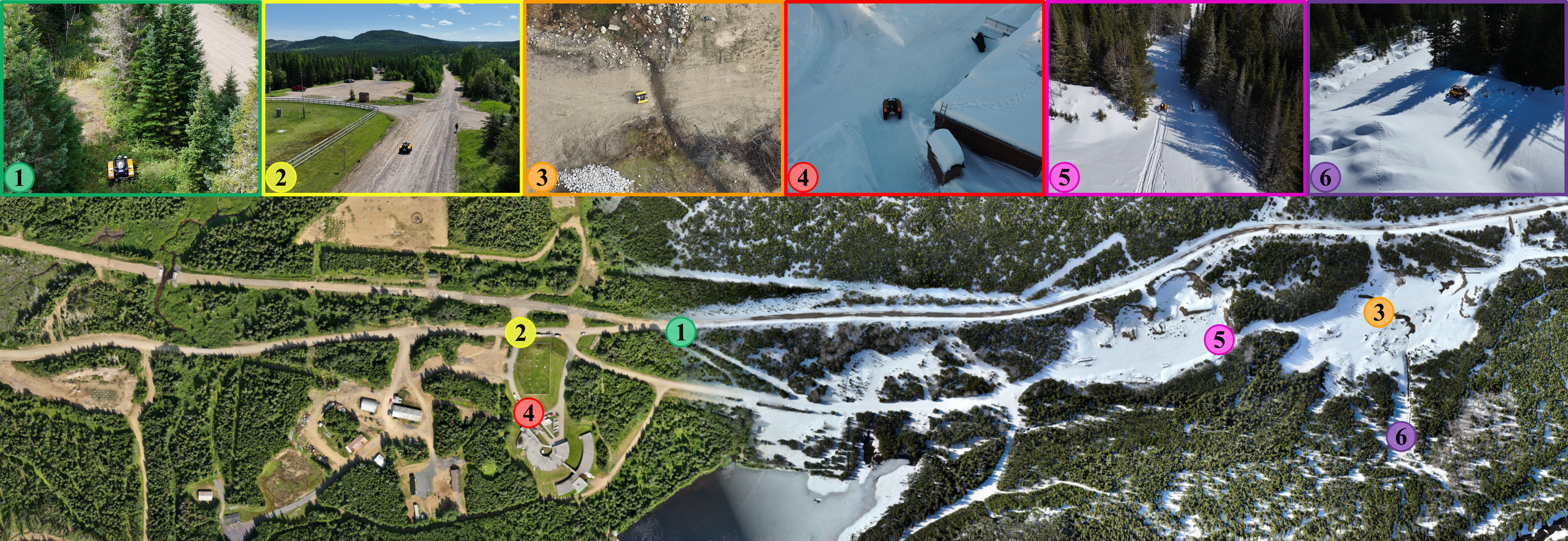
FoMo revisits the same forest routes in all four seasons. Its more than 10 TB of multisensor recordings let researchers test whether a robot can find its way on an old map after the seasons change, well beyond measuring SLAM accuracy on a good day.
 Open full-size image in a new tab
#Tracking motion without a map and finding your place on an old one
Odometry combines successive sensor observations to estimate how far a robot has moved since its last position. Small errors accumulate. Re-localization means finding the robot’s current position on a previously built map. Simultaneous localization and mapping (SLAM) estimates position while building that map. Even in the same forest, snow and changing foliage can make once-familiar features hard to recognize.
Loop closure recognizes a place the robot has already visited and uses it to correct the accumulated trajectory. A small final error can therefore follow substantial errors earlier in a run. FoMo lets us compare the inputs, the corrections each method makes and how much of the trajectory it returns.
#What FoMo adds
Large urban driving datasets feature paved roads and many permanent structures. FoMo revisits six routes through a Canadian conifer forest, including paved roads, unpaved trails and sections with no path. The recordings capture snow over a meter deep, vegetation growth, steep slopes and vibration. The dataset pairs two lidars, FMCW radar, stereo and monocular cameras and two IMUs with reference trajectories derived from three GNSS receivers.
#Numbers and comparison conditions
Twelve deployments over a year covered six routes and more than 64 km, producing over 10 TB. In a cross-season comparison against a January 29 map, lidar–inertial translation drift reached 46.5% on October 14. Stereo–inertial SLAM had 0.9% drift in that comparison but failed to return a complete trajectory in three of nine deployments. The radar–gyroscope method had large average errors with its 2D radar and sharp turns. Each number depends on the sensors used and how often the method failed.
Translation drift averages relative errors over trajectory segments 100, 200 and up to 800 m long in 100 m increments. The 0.9% value describes those segments in one comparison. End-point error and an average across seasons are different quantities. In Table 3 an asterisk marks a trajectory that covered less than 90% of the reference duration. N/A means the trajectory was too short to calculate the metric. Of the three incomplete stereo–inertial runs, two returned partial trajectories and one was N/A. Low error over a short stretch alone cannot establish greater reliability than a method that finished the route.
The appendix attributes the small visual-SLAM error in the October 14 column partly to repeated loop closures. Some methods continued using odometry after re-localization failed. A drift value can therefore reflect both recognition of an old place across seasons and accumulated motion estimates.
#Did the sensors observe the same instant?
Synchronizing the sensors’ clocks and assigning the correct timestamp to an exposure or measurement are two separate tasks. Section 5 independently estimates the delay in the camera driver’s timestamps. Combining observations made at different times while the robot is moving can also misalign them in space.
Equation (1) in the paper estimates this delay.
Equation (1). How late is the driver timestamp? Scroll sideways for long equations. Focus the equation and use arrow keys with a keyboard. Expand symbols and the worked calculation
Express all times in seconds. t_ROS is the driver timestamp, t_QR is the absolute time encoded in the photographed QR code, and t_gen is the time needed to generate that code. Subtracting the reference time, including generation time, from the driver timestamp gives the estimated delay t_delay. The calculation measures a delay. Individual sensors can still have residual latency.
Over 15 minutes the paper reports a mean delay of 51.48 ms with a standard deviation of 8.78 ms. Applying the mean cannot capture every frame’s individual delay. An inertial measurement unit (IMU) measures angular velocity and acceleration. Its driver assigns timestamps as it interprets values received over USB, so the authors estimate IMU latency separately.
Equation (2). Estimating IMU delay relative to the camera Scroll sideways for long equations. Focus the equation and use arrow keys with a keyboard. Expand symbols and the worked calculation
All three symbols denote times. t_imu is the estimated IMU delay, the bar over t_delay denotes the mean camera delay above, and t_shift is the relative time offset estimated by the Kalibr calibration tool. Convert them to common units before subtracting. Section 5 reports 56.09 ms for Vectornav and 60.23 ms for Xsens. Before adding or subtracting either value from timestamps in the data files, check the calibration file’s sign convention for the relative offset.
Kalibr’s official YAML documentation defines timeshift_cam_imu in seconds. Adding that shift to camera time gives IMU time. In the documentation, IMU time is a timestamp attached to an observation. In the FoMo equation, t_imu denotes estimated latency. The convention alone does not establish which files already incorporate a correction or which direction the SDK applies it. That requires checking the files and processing code.
Check your understanding. If the computers’ clocks are synchronized, does that guarantee an accurate camera measurement time? The driver’s choice of when to assign the timestamp and the variation in latency still matter.
#Limitations and counterevidence
#How was the reference trajectory constructed?
The reference trajectory combines postprocessed positions from three GNSS antennas fixed to the robot. Equations (3)–(5) in Section 7 first align the antennas’ known configuration with their measured positions, then estimate the transformation while accounting for uncertainty at each position. A covariance matrix describes how far errors spread in each direction. An ordinary distance measure gives all directions equal weight.
The reference itself also needs validation. A small reported covariance cannot guarantee real-world accuracy. The position and orientation limits described below apply when interpreting this calculation.
Equation (3). An objective that accounts for uncertainty by direction Scroll sideways for long equations. Focus the equation and use arrow keys with a keyboard. Expand symbols and the worked calculation
This objective compares how well different rotations and translations fit the observations. The index k runs over the three antennas. The residual e is the difference between a measured position and the transformed antenna position, in meters. W is that position’s covariance matrix in m². Its inverse W⁻¹ has units m⁻², making each term and their sum J dimensionless. The calculation requires an invertible W.
A displacement of the same size incurs a larger penalty along a direction measured more precisely. In a hypothetical one-dimensional example, a 0.1 m residual contributes 1 when the standard deviation is 0.1 m and 0.25 when it is 0.2 m. These illustrative values show the units and weighting. An inaccurate covariance estimate can give measurements more or less weight than their actual reliability warrants.
Equation (4) finds an initial transformation using unweighted distances between points. Equation (5) describes the estimate that accounts for covariance. The paper says initial alignment is needed for the small-rotation approximation in its point-to-plane method. This review did not trace how the fixed initial residual written in Equation (5) relates to the optimization variable in the implementation. An executable reconstruction would require that check.
Reliance on GNSS favored wider trails, and actual errors beneath the forest canopy can reach tens of centimeters. The paper says the covariance reported by GNSS postprocessing understates the true uncertainty. Small covariance values in the files therefore provide insufficient grounds for assuming millimeter accuracy throughout. The orientation field contains an identity quaternion in place of a reliable orientation estimate. It supplies neither a record of zero rotation nor ground truth for attitude. Heavy snow, battery limitations and access restrictions left some routes incomplete, and the rear camera had an exposure failure. The preliminary benchmark focuses on the Yellow route. A leaderboard covering all sensors and routes is still planned.
#Check your reading
Is the method with the smallest error always the best? Compare the same reference map, evaluation run and extent of trajectory, and count failures separately. Assigning an arbitrary large error to a failed segment would distort the average. FoMo evaluates localization across seasons. Collision-free navigation in every condition is a separate question.
#Code, data and disclosures
codeAvailable: Yes. Python and Rust SDK, with a Docker-based evaluation example.dataAvailable: Yes. Selective downloads, human-readable and ROS2 MCAP formats, calibration, ground truth and RINEX.conflictsOfInterest: The authors declare no potential conflicts of interest.strongestEvidence: Cross-season map reuse exposed both 0.9–46.5% drift and failures to return complete trajectories.limitations: One region and six routes, no reliable orientation in the GNSS reference, the cost of accessing over 10 TB and incomplete repeat runs.
The SDK repository is publicly accessible and its README marks it as a work in progress. Availability, permission to reuse and successful reproduction warrant separate checks. Usage terms for the data, SDK and paper figures must be checked individually. This review did not execute the code or redistribute the data.
#Sources and identifiers
- Full text, arXiv v2 — revised October 5, 2026. Includes the IJRR acceptance statement and DOI.
- Official FoMo dataset — data, SDK and selective downloads.
- DOI
10.1177/02783649261491481, arXiv2603.08433.
#When to revisit
Reassess when the official leaderboard opens, an independent team reproduces the baselines, GNSS orientation or covariance improves, full results across routes and seasons become available, or a smaller distribution package appears.