Start with the practical answer. A test that assigns nearly the same mark to every student is a poor instrument for distinguishing ability. A similar problem can arise when evaluating AI predictions of genetic perturbations. Before changing the model, this study asks whether the metric can distinguish meaningful responses from uninformative predictions. Across 14 datasets and 18 metrics, calibrated evaluation reveals that several deep-learning models outperform simple baselines. It does not establish that every model solves every biological prediction task.[1]
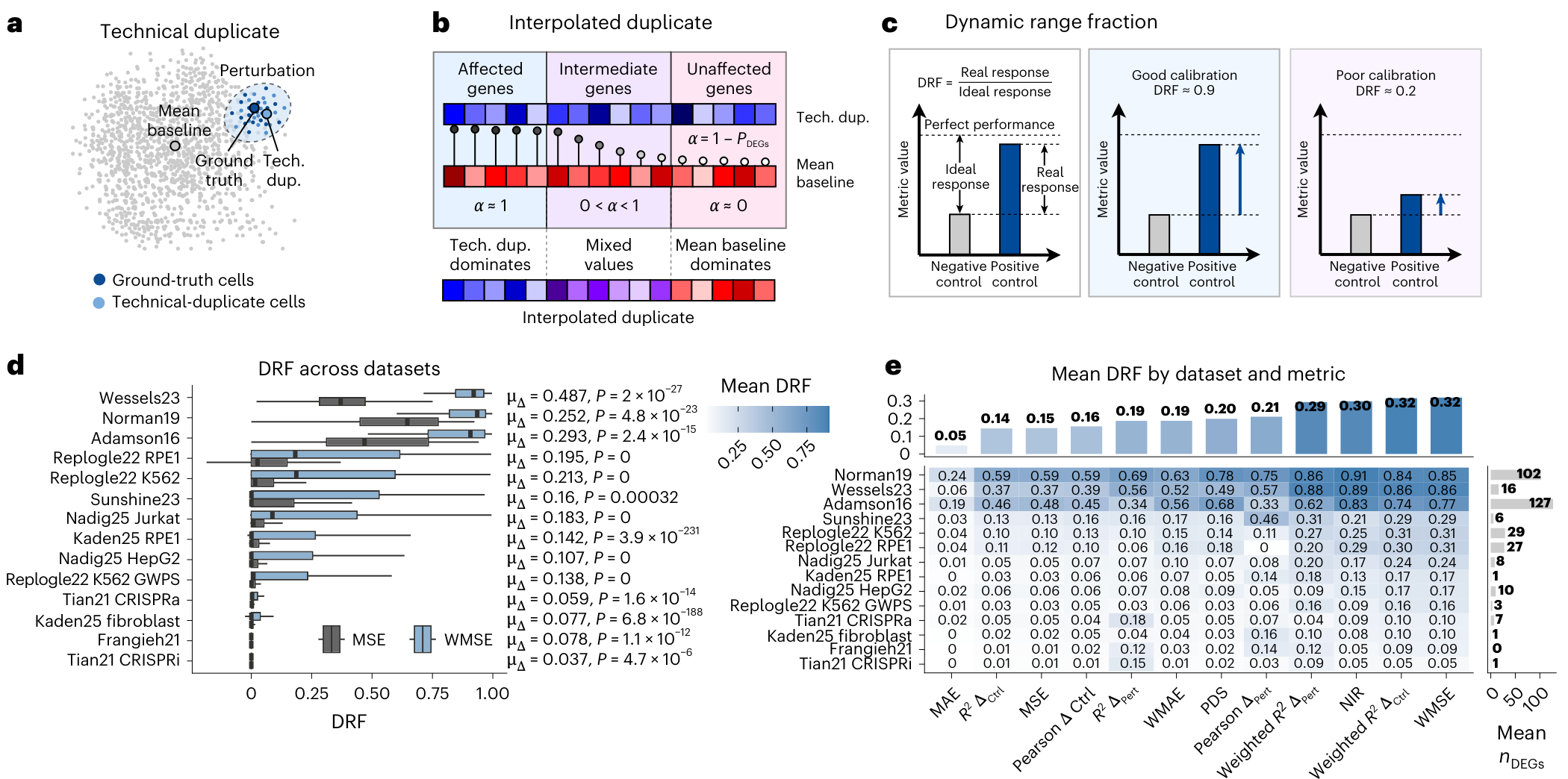
#Reading original Figure 1: inspect the gap between controls first
Panel a divides cells from the same perturbation into two groups and uses one to predict the other. Panel b constructs an interpolated positive control by blending this prediction with a mean baseline on a gene-specific basis. Panel c compares the observed positive–negative control gap with the ideal gap through DRF. Panels d and e examine calibration across datasets and metrics. The plotted calibration values are not drug effects or cell-survival rates.[1]
Start here Perturbations, transcriptomes, baselines and positive controls Open the explanation
A genetic perturbation inhibits or activates a gene to investigate how cells respond. The transcriptome describes which RNA molecules are expressed and at what levels. The prediction target here is this expression response, not an entire DNA sequence or every function of a cell.
A baseline is a simple comparison that a more complicated model should improve upon. Always returning the average perturbed expression profile from training data is easy, but does not understand a particular perturbation’s unique response. A positive control asks whether the metric recognizes predictions containing meaningful information. A control that accesses information about the evaluation perturbation must not be presented as a deployable predictor for previously unseen perturbations.
#1. Two reasons a mean predictor can appear intelligent
Changing one gene does not alter every measured gene by the same amount. If an important response is concentrated in a small subset, an error metric weighting all genes equally can dilute that signal. A mean prediction can score well by matching many unchanged genes while missing the few that matter. The paper describes this as signal dilution.[1]
There can also be systematic changes shared by many perturbed cells relative to controls. Correlation measured against a control reference can then reward recovering those common shifts, rather than recovering what distinguishes a particular perturbation. The paper discusses this as control bias. A high control-referenced correlation should therefore not automatically be interpreted as understanding a perturbation-specific mechanism.[1][2]
What happens to MSE when only a few genes change? Expand symbols and the worked calculation
G is the number of evaluated genes. As a teaching example, suppose ten out of 10,000 genes change by one unit while all others change by zero. Predicting zero throughout misses every affected gene but gives MSE=10/10,000=0.001. These hypothetical values are not a recalculation of any study dataset. They illustrate why a small overall error need not establish recovery of a required biological signal. Normalization, units and the number of affected genes change the actual value.
This is not an argument that MSE is always wrong. Direct error metrics remain useful for detecting implausible expression predictions. The study argues against treating any one metric as definitive and recommends complementary metric families. Choosing only metrics on which a model wins is different from testing metric sensitivity before interpreting model performance.[1]
#2. Why a control with access to relevant information is useful
The researchers used a technical-duplicate control: split cells belonging to a perturbation into two groups and predict one group’s expression using the other. Both groups share perturbation-specific information, so this predictor has relevant information that an unrelated mean baseline lacks. If a metric fails to recognize that advantage, poor model scores cannot be attributed solely to a lack of model capability.[1]
Cellular measurements contain noise, so an average from half the cells is not a perfect prediction. The interpolated-duplicate control blends the technical duplicate with the mean baseline according to gene-level perturbation significance. Strongly affected genes receive more perturbation-specific information, while weakly affected genes receive more of the mean. Understanding this construction prevents treating the positive control as an ideal noiseless measurement.[1][2]
The distinction is between a control used to inspect the evaluation instrument and a model required to predict an unseen perturbation. The positive control can use data from the perturbation being evaluated. Calling it the best deployable model because of its score would change the purpose of the comparison. The study uses it to evaluate metric discrimination, then separately benchmarks prediction of perturbations or combinations held out from training.
#3. DRF measures discrimination, not prediction accuracy
Dynamic Range Fraction (DRF) asks how much of the ideal score gap from a negative control to perfect prediction is occupied by the positive control’s improvement. The expression below can be read in a higher-is-better scoring direction. With loss metrics, the direction of improvement and the implementation’s definitions must be handled consistently.[1]
How much of the available gap does a positive control reveal? Expand symbols and the worked calculation
m is the metric, y the ground truth, and ŷp and ŷn the positive- and negative-control predictions. Epsilon is a small numerical-stability term. For a higher-is-better score, a negative control of 0.90, positive control of 0.91 and perfect score of 1 give approximately 0.1. Scores of 0.20, 0.80 and 1 instead give approximately 0.75. These are teaching calculations, not observed values from the paper. The latter exposes more of the controls’ available separation. If the negative control already approaches perfection, the small denominator can make interpretation sensitive.
DRF is not a model pass mark or a biological safety score. It depends on noise, perturbation strength and control choices. The researchers examined changes in controls, cell counts, sequencing depth and the selection of highly variable genes. These checks also explain why a high DRF from one setting should not simply be copied into a different experimental domain.[1][2]
#4. Separate the calibration dataset collection from the model experiments
The 14 datasets and 18 metrics describe the calibration analysis. They do not mean every model was validated on every generalization task in all 14 datasets. The paper distinguishes unseen single perturbations from unseen combinations and discusses model comparisons in Replogle22 K562, Nadig25 HepG2, Norman19 and Wessels23. Responses in previously unseen cell types, donors or conditions were not evaluated.[1]
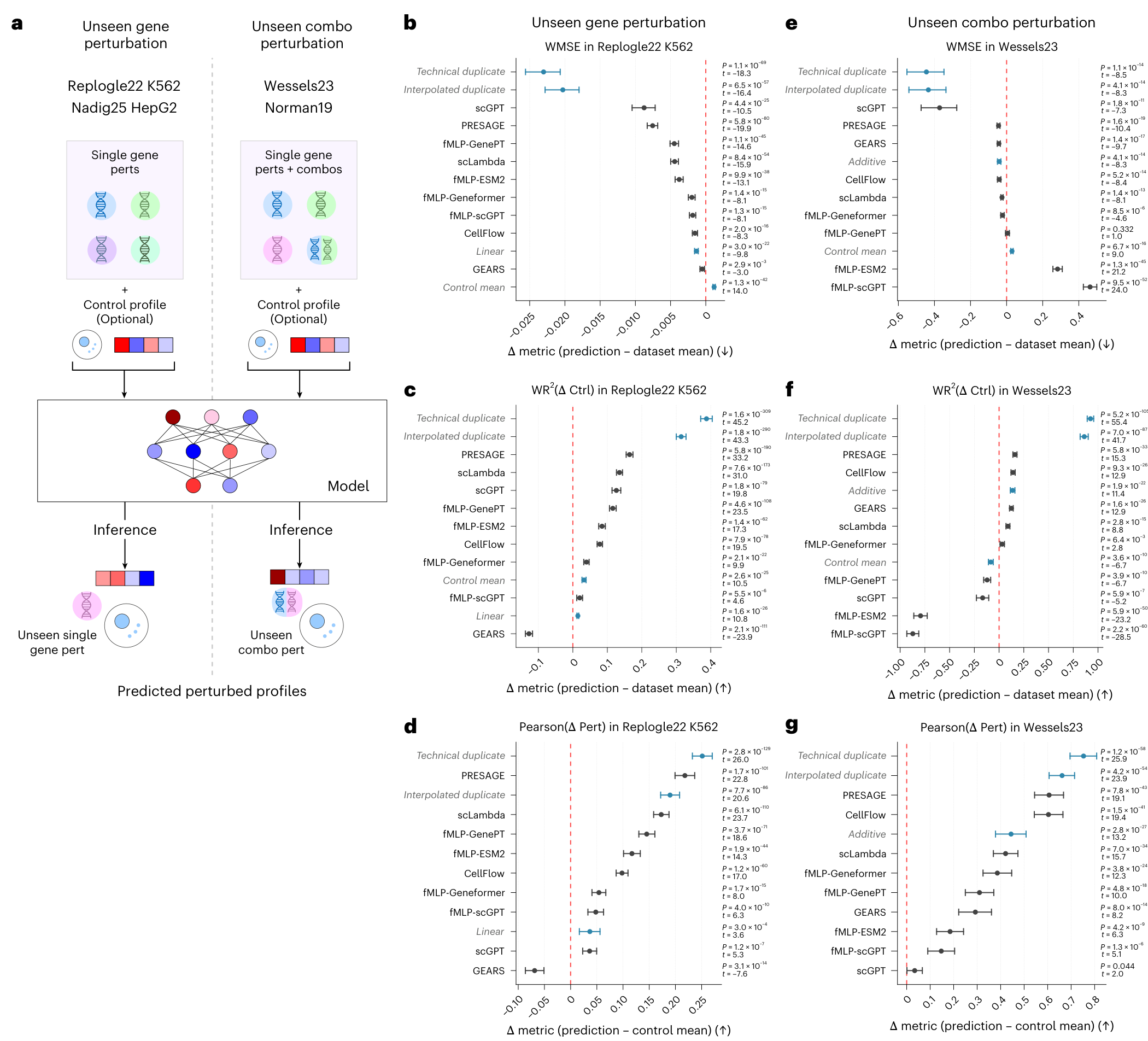
#Reading original Figure 2: a winner depends on the question
Panel a distinguishes the training and test arrangements for single and combined perturbations. Panels b–d cover single-perturbation prediction, while e–g cover combinations under different metrics. Some horizontal axes express differences from a baseline, and direct errors are better when smaller, so read the axis direction first. Error bars and comparison groups also matter. A favorable position in one panel does not establish superiority under every objective.[1]
Models include scGPT and GEARS, more recent PRESAGE, scLambda and CellFlow approaches, and MLP probes using embeddings from several foundation models. Performance of a predictor supplied with an embedding should not be relabeled as direct perturbation prediction by the foundation model itself. Architectural family, version, adaptation and evaluation metric all contribute to the experimental setting.[1]
| Question | Evidence or observation | Interpretation not established |
|---|---|---|
| Can metrics distinguish the controls? | Calibration across 14 datasets and 18 metrics | Guaranteed performance for every cell/model combination |
| Did earlier models contain useful signal? | Several models exceed uninformative baselines under calibrated metrics | Superiority of every model on every metric |
| How much combination space is exposed in training? | Norman19 coverage of 0.63% | Representation of all biological combinations |
| What happens with greater coverage? | PRESAGE exceeds additivity on 15 of 18 Wessels23 metrics | Generalization to arbitrary combinations and cell contexts |
| Is practical benefit established? | Associations with pathway and neighborhood recovery | Proven treatment effects or clinical outcomes |
#5. When a simple additive baseline is already close to saturation
Predicting a two-gene perturbation by adding the effects of its single-gene perturbations is a simple but strong baseline. Many effects in Norman19 are additive, and this study’s training set covers 31 of 4,950 possible pairs, approximately 0.63%. This creates limited opportunity to learn nonadditive interactions, while the additive baseline can already occupy much of the ideal performance gap.[1]
Wessels23 exposes 10.3% of its possible combinations during training. In that setting, several models exceed the additive baseline on selected calibrated metrics, and PRESAGE exceeds it on 15 of 18 metrics. The fraction 15/18 must not be converted into an 83.3% cellular-prediction success rate. It counts metrics, not successfully predicted cells or samples.[1]
The two datasets are not a controlled experiment differing only in coverage. Gene counts, perturbation strength and experimental context also differ. Their contrast supports the relevance of combination exposure but does not prove that coverage alone causes every performance difference. The paper explicitly identifies evaluation on additional combinatorial datasets as a remaining need.
#6. What an exclusively optimistic interpretation would miss
The study does not declare every previous negative benchmark conclusion wrong. It presents evidence that some metrics can obscure predictive information by failing to distinguish it clearly. Even among calibrated metrics, model rankings differ with the objective. Reconstructing overall expression, recovering relative changes and retrieving the correct perturbation are not identical tasks.[1]
An evaluator should therefore avoid looking at the models first and selecting only favorable metrics afterward. A more convincing design specifies intended applications, positive and negative controls and multiple metric families in advance. Substantial underperformance on direct error metrics cannot be dismissed merely because their calibration is lower; they can still flag biologically implausible predictions.
The study also leaves unseen cell types, donors and conditions unaddressed. Predicting a new genetic perturbation in a familiar cell system differs from predicting a response in a new patient’s tissue. Accurate transcriptomic prediction in experimental data does not establish a drug’s safety or a treatment’s benefit in people.[1]
#7. Disclosures and the design of the next benchmark
The paper discloses that several authors are Shift Bioscience employees and that Bo Wang is Chief Artificial Intelligence Scientist at Xaira Therapeutics. These are publication-time disclosures, not a separate investigation of every author’s current role. They do not automatically invalidate the result; they provide context for evaluating transparent code, processing decisions, model versions and independent reproduction.[1]
Reproduction code is available in the official repository. This explainer did not retrain every model or download and recompute all 14 datasets. Individual model licenses, including conditions applying to PRESAGE, do not disappear because the benchmark repository is convenient to access. Public code, an actual reproduction run and clinical validation are different completion states.[3]
Future tests should examine the same calibration principles across additional combination datasets, new cell contexts and changes in noise or sample size. Rather than forcing distinct evaluation objectives into one score, reporting how clearly the positive control separates from the negative control helps distinguish a model’s failure from an insensitive test. The contribution is not that AI can predict everything, but that the instruments used to judge AI also require validation.
#Sources and access scope
[1] Miller et al., Deep learning perturbation models can outperform baselines on calibrated metrics, Nature Biotechnology, 1 October 2026, DOI 10.1038/s41587-026-03307-w. Publisher.
[2] Supplementary Notes 1 and 2: controls, metric calibration and additional analyses of data quality and selection. Supplement.
[3] Shift Bioscience, Perturbation-Models-Outperform-Baselines, the official reproduction repository. Code.
The edition date is 2 October 2026; source, figure and license checks took place on 5 October. The publisher’s final article and PDF and relevant supplementary passages were checked. Original Figures 1 and 2 retain their complete panels, axes and annotations, with attribution under CC BY 4.0. The supplied score of 97 and previous candidate-search scope are editorial records, not a newly calculated scientific probability or a discovery scan repeated here. No individual diagnosis, treatment recommendation or independent model retraining was performed.