A 25,000-hour SOEC stack: durability through operating control

A 70-cell SOEC, alternating operating directions and voltage histories — **Original Figure 1** Panel a shows the stack and cell, b the alternating operating directions, c early DC operation, and d the long voltage and temperature history. Panels c and d have different voltage-axis ranges. The 0.05%/kh figure applies to the later 22,268-hour window. Bilalis et al. · Nature Communications · Figure 1 · Source · CC BY-NC-ND 4.0 · PNG rendering preserves all original figure panels, axes and annotations; surrounding article text is excluded. No redraw or color inversion.

#1. The conclusion starts with the measurement window

A longer-lived solid oxide electrolysis cell (SOEC) stack does not necessarily require a new electrode material. The researchers operated a 70-cell industrial stack using AC:DC operation, inserting short fuel-cell intervals into predominantly electrolytic operation. The complete analysis window spans 25,011 hours. The much lower reported voltage degradation of 0.05% per 1,000 hours applies to a later 22,268-hour window. Calling it “0.05% throughout 25,000 hours” erases a central qualification.[1][2]

The paper was released on 24 September 2026 as a peer-reviewed, accepted early version with a permanent DOI. The authors describe it as the longest and lowest-degradation full-stack operation known to them. That is a qualified comparison with the literature, not a certification covering every manufacturer’s product and every operating condition. This explainer separates the strength of the endurance observation from the causal effect attributed to the control strategy.[1]

#2. Why lifetime can constrain an efficient electrolyzer

Splitting water into hydrogen and oxygen requires energy. SOEC uses high-temperature steam so that heat can supply part of that requirement. This can reduce the electrical contribution, but it does not make the heat free. Electrical efficiency and total energy efficiency have different accounting boundaries. A low electricity figure alone cannot establish the lowest hydrogen cost while omitting steam production, the heat source, and balance-of-plant power.

A stack is also not just a single cell made larger. Gas must reach many cells evenly, while seals, contacts and current paths remain functional. Local reactant starvation or overheating can occur even when the average temperature looks acceptable. Changes in electrode connectivity and interfaces alter the paths taken by current. Needing a higher voltage to maintain the same current is the practical meaning of voltage degradation.[1][2]

At constant current, electrical power is voltage multiplied by current, so a rising voltage generally increases the electrical burden. Nevertheless, voltages measured at different temperatures, gas compositions or current densities do not isolate damage. Reversible changes in operating point must be distinguished from irreversible degradation. For an endurance record, what was held constant—and when conditions changed—is as important as elapsed time.

#3. Designing the current waveform rather than replacing materials

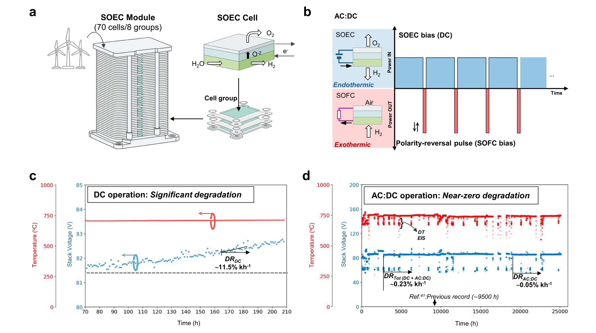
Improved electrodes, electrolytes and protective coatings remain important. This study does not make materials engineering unnecessary. It adds another design variable: the time pattern of the current supplied to the same stack. Rather than maintaining only the electrolysis direction, brief reversals periodically change electrode polarization and heat generation.[1]

Electrolysis and fuel-cell operation drive opposite reaction directions. The term AC should not be confused with a symmetric alternating waveform that produces no net hydrogen. The waveform retains a mean bias toward electrolysis. Short fuel-cell intervals can coexist with net electrolytic operation over a full cycle. Frequency, current amplitudes, switching time and mean current therefore need to be read together.[2]

The expression below is an explanatory two-state average, not a claim that the experimental supply generated a perfectly rectangular waveform. D is the fraction of each cycle spent in electrolysis; the sign convention takes electrolytic current as negative.

\bar I=D I_{\mathrm{EC}}+(1-D)I_{\mathrm{FC}},\qquad I_{\mathrm{EC}}<0<I_{\mathrm{FC}}\tag{1}

Increasing the reversal frequency alone does not guarantee better operation. The two current amplitudes and their time fractions also determine mean current and heat generation. The reported 30 Hz is a condition used for this stack and its supply, not a universal setting that can simply be copied into any plant. The engineering problem combines thermal, gas-flow and electrical control.

#4. What was actually operated at stack scale

The experiment used 70 cells, each with an active area of 80 square centimetres. The fuel electrode was Ni–YSZ, the electrolyte approximately 8–10 micrometres of 8YSZ, and the oxygen electrode an LSCF/ceria-based structure. The principal long-term period used an inlet temperature around 750°C and an average electrolytic current density around −0.5 A per square centimetre. This differs substantially in scale and duration from a short accelerated experiment on a small single cell.[2]

The supplement reports operation primarily at 30 Hz, corresponding to a cycle of approximately 33 milliseconds. A Regatron G5.RSS bidirectional supply switched the operating direction in less than a millisecond. Gas supply, temperature control and voltage monitoring were integral parts of the arrangement. The result consequently does not establish that adding arbitrary alternating current to an existing rectifier will reproduce the same endurance.[2]

In the first original figure, panel a describes the stack and cell, panel b the alternating operating directions, panel c the early DC interval, and panel d the long-duration voltage and temperature history. The voltage-axis ranges differ between panels c and d. Their apparent slopes cannot be compared by eye without respecting those scales. Table S2 provides the appropriate window lengths and endpoint voltages; the long graph also includes diagnostic interruptions and operating changes.[1][2]

#5. Recalculating the headline numbers

Supplementary Table S2 defines the overall window from hour 70 to hour 25,081, a difference of 25,011 hours. The stabilized period extends from hour 2,813 to hour 25,081, or 22,268 hours. The endpoint voltages below are rounded values from the table. Each relative rate is normalized by the starting voltage of its own window.[2]

Analysis window	Duration	Initial → final voltage	Reported relative degradation
Overall window	25,011 h	81.4 → 86.2 V	0.23%/kh
Later long AC:DC period	22,268 h	85.2 → 86.2 V	0.05%/kh
Intermediate DC interval	596 h	91.2 → 91.1 V	Listed as 0.0%/kh

One kh means 1,000 hours. The relative degradation calculation is an endpoint-based normalization. Changing either the initial voltage or the duration changes the calculated rate.

DR=\frac{V_f-V_i}{V_i}\frac{1000\ \mathrm{h}}{t_f-t_i}\times100\%\tag{2}

Using the rounded late-period endpoints gives 1.0 V divided by 85.2 V and 22.268 kh, multiplied by 100: approximately 0.0527%/kh. The overall-window calculation gives approximately 0.2358%/kh. These support the scale of the reported 0.05 and 0.23 values. This is a recalculation from the table, not a new digitization of the graph. The window definition matters much more than the last reported decimal place.

The approximately 0.65 mV/kh per-cell figure also describes the later regime. Dividing the rounded stack-voltage increase by duration and 70 cells gives approximately 0.64 mV/kh; rounding of endpoints explains a small difference. Conversely, linearly extrapolating 0.05%/kh to claim decades of guaranteed operation exceeds the evidence. A window-averaged voltage drift is not a failure probability or a distribution of remaining useful life.[1][2]

#6. Evidence beyond a flat voltage trace

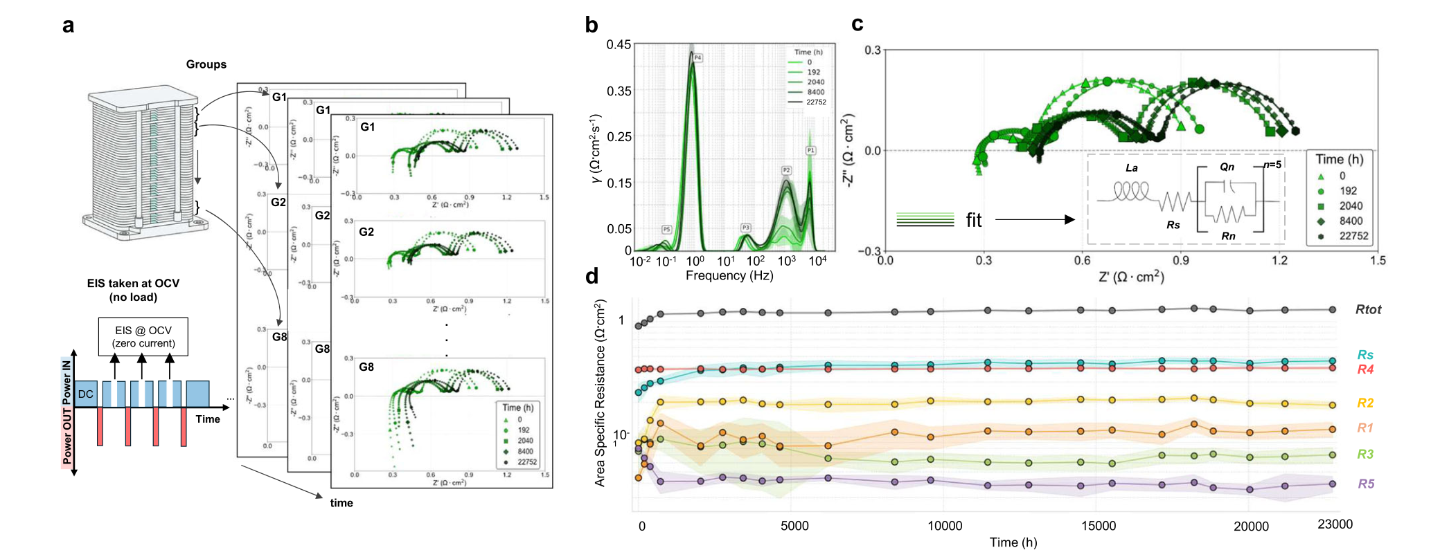
Cell-group impedance and changes in resistance components over time — **Original Figure 2** Panel a links cell groups to Nyquist responses, b shows relaxation-time distributions, c equivalent-circuit fitting, and d resistance histories. These complement voltage evidence but do not uniquely assign every resistance element to one damage mechanism. Bilalis et al. · Nature Communications · Figure 2 · Source · CC BY-NC-ND 4.0 · PNG rendering preserves all original figure panels, axes and annotations; surrounding article text is excluded. No redraw or color inversion.

The authors combined voltage measurements with electrochemical impedance spectroscopy (EIS) and post-test cross-sectional examination. EIS measures the response to a small perturbation over frequency, helping distinguish processes operating on different timescales. A point on an impedance plot, or an element of a fitted equivalent circuit, does not automatically identify one unique damage mechanism.[1][2]

In the second original figure, panel a links monitored cell groups to representative Nyquist responses; panel b examines distributions of relaxation times; panel c illustrates equivalent-circuit fitting; and panel d tracks resistance components over time. Monitoring multiple groups matters because a stable average voltage could otherwise conceal increasing heterogeneity. Each panel has its own axes and units, which should be read before drawing a physical interpretation.[1]

Supplementary Table S5 reports a total-resistance increase of approximately 0.23 Ω cm²/kh initially and 0.001 Ω cm²/kh later. The table also reports dispersion, so the small late mean must not be read as proof of absolute zero degradation. Post-test examinations considered nickel connectivity, interfaces and contamination signatures. These observations support stabilization, but a limited set of cross sections cannot exclude every possible defect throughout a stack.[2]

Similarly, an element not being clearly detected within a method’s detection limits is not proof that no atoms of that contaminant exist. The value of combining EIS with microscopy is that they constrain different aspects of the interpretation. Their agreement still does not turn a study without a separate matched endurance control into definitive evidence of a single cause.

#7. Counterevidence and limits of the comparison

The central limitation is the absence of two otherwise matched stacks run in parallel for 25,000 hours, one DC-only and one AC:DC. Early DC operation differs from later operation in chronology, temperature and conditioning history. Manufacturing quality, gas purity, the power supply and thermal management can contribute simultaneously. The paper itself recognizes possible contributions from stack quality and the robustness of the experimental arrangement, not just the waveform.[1][2][3]

The intermediate 596-hour DC interval is a particularly important counterexample to an overly simple story. Its rounded endpoint voltage decreased slightly, from 91.2 to 91.1 V, and the table lists a zero rate. Thus, “DC always immediately causes rapid deterioration” is inconsistent with the reported data. Conversely, a short interval at different conditions does not invalidate the long AC:DC observation. A short operating window and a long endurance experiment answer different questions.[2]

Earlier literature benchmarks are not same-product comparisons conducted under one protocol. Cell counts, areas, temperatures, current densities and gas conditions vary. “About an order of magnitude lower” refers to reported long-duration stack results, not a randomized treatment effect. The observed persistence of low drift and the fraction of that persistence caused specifically by AC:DC must remain separate propositions.[1][2]

#8. What is still needed to connect durability to hydrogen cost

Lower voltage drift could reduce long-run electrical consumption and replacement costs. Yet bidirectional conversion is not lossless. Recovering or consuming energy during reverse pulses, generating steam, recirculating gas, heating and auxiliary loads all belong in a clearly stated system boundary. The following expression explains that accounting boundary; it is not a measured commercial-plant result from the paper.

e_{\mathrm{sys}}=\frac{E_{\mathrm{grid,net}}}{m_{\mathrm{H_2,net}}}\quad[\mathrm{kWh\,kg^{-1}}]\tag{3}

Net electrical input means imported electricity minus electricity returned across the same boundary; the denominator is actual net hydrogen production. Mixing measurements at the converter output with measurements at the grid meter can make conversion losses disappear on paper. If heat is supplied outside the electrical boundary, its energy and cost must be disclosed separately. Improved rectifier efficiency, reduced electrode degradation and reduced whole-system kWh per kilogram are therefore distinct findings.

The supplementary economic assessment depends on assumptions about plant scale, electricity price and utilization. It should not be presented as a commercially achieved hydrogen price. Some authors are affiliated with DynElectro and SolydEra, as disclosed in the paper. That does not automatically invalidate the work, but it strengthens the importance of transparent conditions and independent replication.[1][2]

#9. The next milestone is reproducibility, not just more hours

A priority follow-up is long-duration parallel operation against a DC-only stack from the same manufacturing batch. Average temperature and current density are not the only matching variables: steam utilization, startup history, electrical losses and measurement methods also matter. This would more tightly separate a waveform effect from differences in the test environment. Reporting individual stack outcomes, interruptions and failures would help reveal variation hidden by averages.

Further checks should include higher current densities, multiple stacks and manufacturing variation, renewable-power ramps and repeated restarts. Finally, net hydrogen output and the combined energy and replacement burden must be compared within the same system boundary. A single trace beyond 30,000 hours would be useful, but independent reproduction across products and sites would be more informative for industrial standardization.

The defensible conclusion is that operating control can be a major design variable for long-term SOEC degradation, even without replacing the electrode chemistry. This is neither a universal substitute for materials research nor a demonstrated commercial cost revolution. Preserving the distinctions between long observation, late-window drift, convergent diagnostics and remaining control/efficiency gaps makes the actual contribution clearer.[1][2]

#Sources and access scope

[1] Bilalis et al., Record stack durability in industrial solid oxide steam electrolysis through operational control, Nature Communications, published 24 September 2026, DOI 10.1038/s41467-026-78001-1; accepted early version. Original source.

[2] Supplementary Information to the same paper: Note 2 operating conditions, Note 3 and Table S2 degradation windows, Table S5 resistance changes, post-test microstructure and economic assumptions. Original source.

[3] Transparent Peer Review file: reviewer comments and author responses on comparisons and interpretation of the operating strategy. Original source.

Checked on 25 September 2026 against the publisher’s accepted early-version PDF, the operating conditions and Tables S2/S5 in its supplement, and the peer-review record. The citable, peer-reviewed early version may be replaced by the edited Version of Record. No independent endurance experiment or hydrogen-cost replication was performed. Reproduced figures retain all original panels and carry attribution and CC BY-NC-ND 4.0 notices; this explainer page does not display advertising.