Learning that a motor has failed only after it stops is too late. Production has already stopped, and components may already be damaged. Prognostics and health management (PHM) uses equipment signals such as temperature, current and vibration to diagnose the current condition, monitor developing anomalies and, where possible, estimate remaining useful life.
In 2024, as an undergraduate researcher, I helped a master’s student in my laboratory with research involving motor vibration data. In 2026 I revisited the data description and Python code from that work. I used our presentation to reconstruct the preprocessing exercise and reviewed a separate document, A Study on Fault Diagnosis, for background on PHM and fault diagnosis in robot reducers. The original data are private. The figures and numbers below describe that particular experiment.
What the review found. The pipeline was a useful exploratory exercise: it read large CSV files, applied interquartile range (IQR) clipping and scaling, and ran principal component analysis (PCA) and t-distributed stochastic neighbor embedding (t-SNE). Visually distinct clusters in two dimensions are insufficient evidence of successful fault diagnosis. A diagnostic model needs validation on new measurement sessions, with operating conditions accounted for and labels excluded from the inputs.
#An introduction to PHM
Damage to a bearing or gear in a rotating machine changes friction and impacts. A sensor records those changes as a vibration signal over time. The aim is to identify patterns characteristic of a fault that recur across operating speeds and loads. A large number by itself tells us little.
Equipment and operating conditions
  ↓
Sensor measurements
  ├─ Time waveform → RMS, peak, crest factor → vibration magnitude and impulsiveness
  └─ FFT/frequency features → rotation, gear and bearing components
  ↓
Condition diagnosis / anomaly detection / life prediction
PHM encompasses three questions.
| Question | Task | What this experiment covered |
|---|---|---|
| Is the machine operating normally? | Anomaly detection | PCA and t-SNE as an initial exploration of structure |
| What failed? | Fault classification and diagnosis | Requires separate labels and a validated model |
| How much longer can it operate? | Prognostics and remaining useful life estimation | No degradation timeline was available for this task |
This work therefore covers exploration and preprocessing for vibration-based diagnosis. It stops short of a complete fault prognostics system.
#Reconstructing the data structure
The presentation records the following features in one row from the SVS 40 vibration sensor.
| Feature group | Count | Interpretation |
|---|---|---|
| Time Peak | 1 | Largest amplitude during the observation window |
| Time RMS | 1 | Representative magnitude associated with vibration energy |
| Crest Factor | 1 | Peak / RMS, indicating the prominence of a transient impact |
| Time Data | 2,048 | Raw waveform samples in time order |
| FFT Data | 1,024 | Frequency components obtained from the waveform |
| Total | 3,075 | Sensor features, excluding settings and labels |
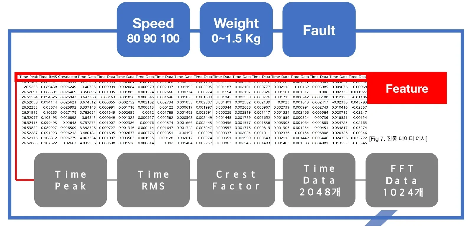
Experiment design, adapted for the web from slide 10 of the AML lab presentation of February 6, 2024. The three blue boxes identify the operating speed (80, 90 or 100), load (0–1.5 kg) and fault condition. Under the sample data row, the gray boxes list peak, RMS, crest factor, 2,048 waveform samples and 1,024 FFT values. These add up to 3,075 sensor features.
Speed and load are more than incidental metadata. Even a healthy motor’s vibration distribution changes with speed and load. A model that memorizes speed 100 as a proxy for fault can perform well on the training data. Record at least the following separately.
- Sensor position and sensor ID
- Rotational speed and load
- Healthy or faulty condition and fault type where known
- Measurement date and run or session ID
- Sampling rate, window length and overlap
- Equipment replacement, remounting or gain changes
#How the background document relates to this experiment
A Study on Fault Diagnosis relates to the master’s student’s research that I supported as an undergraduate. I do not claim the entire study as my own. It examines an industrial robot’s harmonic drive under normal, flexspline defect and backlash conditions and compares a vibration sensor with a three-axis accelerometer.
The Python files and presentation, by contrast, directly document a separate preprocessing exercise that read sensor groups such as H, B and F, speed and load from filenames. The PDF provides background on PHM experiment design. The presentation and code document the preprocessing and exploration I contributed to. I kept the two sources’ operating conditions and labels separate.
#Interpreting vibration features physically
#RMS and overall vibration energy
For a waveform x of length N, root mean square (RMS) is
RMS = sqrt((x₁² + x₂² + ... + xₙ²) / N)Higher RMS can indicate greater vibration energy. Increased speed or load can also raise RMS, so compare it against a healthy baseline for the same operating condition before attributing the change to a fault.
#Peak and crest factor for transient impacts
Peak is the largest absolute value in the window. Crest factor is Peak / RMS. A defect that causes repeated impacts can affect crest factor before RMS changes substantially. A sensor hitting a table or a poor cable connection can also cause a single large peak. Inspect the time waveform to distinguish an equipment event from a measurement artifact.
#FFT and repetition at particular frequencies
The fast Fourier transform (FFT) gives frequency components of a time waveform. Their amplitudes can be compared at rotational, gear mesh and bearing defect frequencies and at their harmonics. To convert 1,024 FFT bins into physical frequencies in hertz, we need the sampling rate and window length. Without this metadata we can still plot the bins, but their physical interpretation is limited.
#What the Python code actually did
| Stage | Implementation found | What worked | What to improve |
|---|---|---|---|
| Input checks | Counted rows and accumulated memory usage using read_csv(..., chunksize=1000) | Recognized the risk of loading files around 16 GB at once | Recombining all chunks still drives up peak memory |
| Schema assignment | Applied column names from a separate Excel file to the CSV | Gave meaning to unnamed sensor columns | No validation of column count, dtype or units |
| Metadata | Parsed sensor, speed and weight from filenames | Linked operating conditions automatically | Could silently accept malformed filenames |
| Feature combinations | Compared all features, FFT only, and FFT plus peak, RMS and crest factor | Explored contributions from feature groups | No retained table of results by condition or selection criteria |
| Outliers | Used 1.5×IQR clipping within time and FFT segments of each row | Examined the effect of extreme values | Could clip genuine fault impulses |
| Scaling | Compared MinMaxScaler, StandardScaler and no scaling | Treated preprocessing as an experimental variable | Fitting before splitting leaks test information |
| Dimensionality reduction | PCA retaining 99% of variance or 12 components, followed by 2D t-SNE exploration | Explored high-dimensional structure | Possible label contamination and incomplete records of seeds and sampling |
The presentation concluded that, depending on the data, scaling and outlier removal could suppress informative features. That is a useful starting point for controlled comparison. Evaluate raw, clipped, standardized and normalized inputs on the same data split before choosing a method.
The original and revised code are linked below. The archive preserves the original absolute paths and experimental remnants. The archived scripts were not packaged for immediate execution.
- Code archive notes
- Revised IncrementalPCA pipeline
- Original preprocessing code
- File merging code
- Original PCA code
- Original t-SNE code
#Reading the three result plots again
#A PCA plot that suggests label leakage
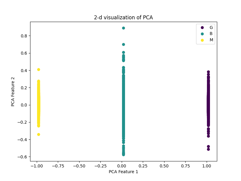
The yellow M points line up near −1 on the first PCA axis, teal B near 0 and purple G near +1. Values vary vertically within each group but barely move horizontally.
The three G/B/M groups lie almost exactly at -1, 0 and 1 on the first axis. It is difficult to explain three such distinct vertical lines using natural vibration features alone. A numerically encoded category or another column directly reflecting the label likely remained in the PCA inputs.
The plot is evidence of a possible target leakage failure. The PCA input matrix should contain sensor features alone. Keep label, sensor, speed and weight as metadata for coloring points and defining validation groups.
#PCA with sensor features
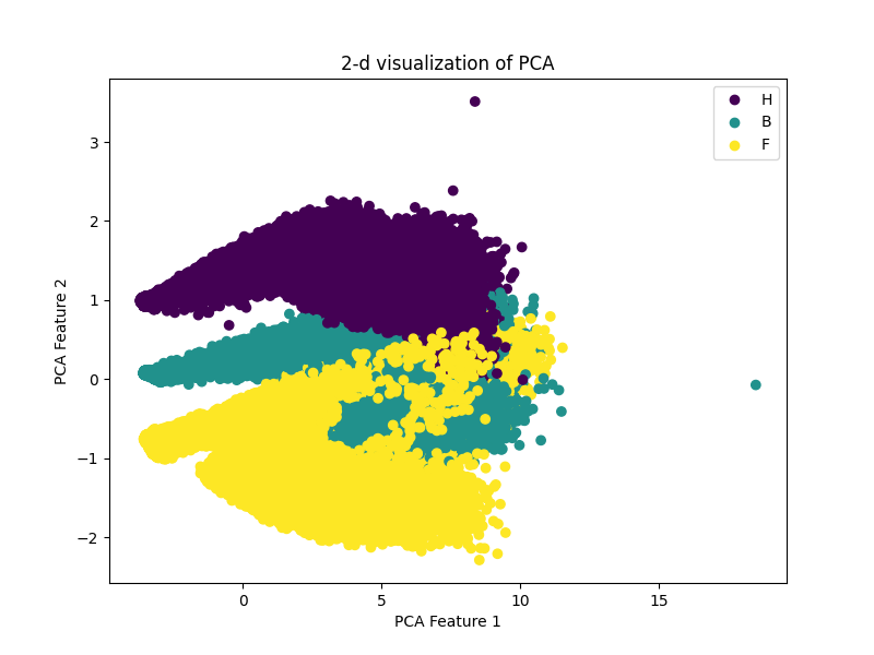
The upper band is largely H (purple), the middle band B (teal) and the lower band F (yellow). Toward the right, the distributions overlap. The axes are principal component scores.
The H, B and F groups form curved regions with overlapping boundaries. PCA finds orthogonal directions of high variance across the inputs. It does not optimize for class separation. The plot alone cannot distinguish mounting position, gain, speed, load or a real fault pattern as the cause of the separation.
Two controlled comparisons would help.
- Compare sensors or conditions at the same speed and load.
- Compare speeds and loads for the same sensor and condition.
The recorded explained-variance ratio of approximately 0.7861 for the first principal component means that 78.61% of the sample variance across input variables lies along that linear axis. It does not mean that 78.61% of the fault is explained. A small impact signal important to a fault can lie along a low-variance direction.
#Reading a t-SNE map
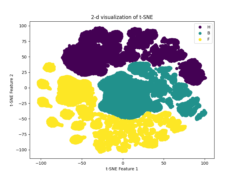
The purple H samples occupy several upper clusters, the teal B samples cluster through the middle and right, and the yellow F samples extend to the left and below. The islands show the arrangement in this embedding. Axis values and distances between distant islands have no direct physical units.
The three groups split into multiple islands. t-SNE optimizes for nearby neighbors to appear close in two dimensions. Perplexity, random seed, learning rate and sample selection can all change the shape.
At most, this plot suggests that some local neighborhoods differ. Classification and anomaly detection performance still need to be measured on separate, unseen measurement sessions.
#The largest leakage risk: randomly splitting rows
Vibration datasets often divide a continuous recording into many short windows. Adjacent windows share almost identical operating states and noise. A random row split can place near-twins from the same measurement in both training and testing.
Row split that leaks session information
session A: [window 1 → train] [window 2 → test] [window 3 → train]

Session-level split
train: sessions A, B, C
valid: session D
test : session E  ← held out until preprocessing selection and tuning are complete
For repeated measurements of one motor, use the session or run ID as the group in GroupKFold. If deployment will involve different motors, split by motor ID to assess that harder generalization problem.
#Redesigning IQR outlier handling
The IQR fences are Q1 - 1.5×IQR and Q3 + 1.5×IQR. The presentation and code used capping, replacing values outside the fences with the nearest boundary. This can be reasonable for tabular data, but extreme vibration values can be the very impacts that reveal a defect.
- Check the sensor’s measurement limits and saturation.
- Determine whether a spike occurred once or recurs on every rotation.
- Look for a corresponding component in the FFT, envelope spectrum or order spectrum.
- Compare raw, IQR-capped and robust-scaled inputs on the same split.
- Finalize the processing rule before examining the test results.
A point outside a box plot fence is a statistical observation. Attributing it to sensor noise requires engineering evidence.
#Reconstructing a reproducible pipeline
from pathlib import Path
import pandas as pd
from sklearn.decomposition import IncrementalPCA
from sklearn.preprocessing import StandardScaler

META = ["sensor", "speed", "weight", "session_id", "condition"]

def iter_chunks(paths: list[Path], schema: list[str], chunksize: int = 10_000):
    for path in paths:
        labels = parse_and_validate_filename(path.name)
        for chunk in pd.read_csv(path, header=None, names=schema, chunksize=chunksize):
            if len(chunk.columns) != len(schema):
                raise ValueError(f"schema mismatch: {path.name}")
            yield chunk.assign(**labels)

# 1. Split the measurement sessions before working with individual rows.
train_files, valid_files, test_files = split_by_session(all_files)

# 2. Fit the scaler and PCA on training data only.
scaler = StandardScaler()
ipca = IncrementalPCA(n_components=12, batch_size=10_000)

# 3. Select preprocessing and the model on validation data, then evaluate the test set once.
The chunksize option alone does not keep memory use low. Recombining all chunks into a giant DataFrame loses the benefit. Accumulate statistics in a stream, apply IncrementalPCA with partial_fit on chunks, and write partitioned outputs in a column-oriented format such as Parquet.
#Figures for the next experiment
| Figure | What to inspect | How to avoid misinterpretation |
|---|---|---|
| Raw waveform and zoomed segment | Impact magnitude and recurrence | Match y-axis scales and label speed and load |
| FFT or power spectral density (PSD) | Frequencies of recurring components | State the sampling rate and label the axis in Hz |
| RMS and crest factor distributions | Energy and impulsiveness by condition | Show individual session points too |
| PCA scores and loadings | Variance structure and contributing features | Exclude label columns and report explained variance |
| t-SNE or UMAP | Local neighborhoods | Record the seed, sample count and parameters |
| Confusion matrix | Which faults the model confuses | Use fully held-out test sessions |
| Alarm timeline | Field false alarms and detection delays | Separate the time interval used to set the threshold |
Report more than accuracy. When faults are rare, include PR-AUC and recall for each class. For deployment, also measure false alarms per hour and detection timing relative to failure.
#Checklist for a repeat experiment
- Fix column names, units and sampling rate in a data dictionary.
- Save sensor, motor, run and session IDs with the data.
- Count samples for each combination of condition, speed and load.
- Audit missing and infinite values, constant columns and duplicate windows.
- Split training, validation and testing by session or motor first.
- Fit the scaler, PCA and feature selection only on training data.
- Measure a confounder baseline that predicts using speed and load alone.
- Compare raw and IQR-processed inputs on the same split.
- Check the physical meaning of PCA loadings and frequencies.
- Record t-SNE seed, perplexity and sample selection.
- Report per-class precision, recall, F1 and PR-AUC alongside accuracy.
- Preserve library versions, seeds, run commands and result tables.
#What the records establish and what remains unknown
The records establish the 3,075-feature SVS 40 structure, the speed and load conditions, plans for comparing IQR processing, scaling and feature sets, and the historical PCA and t-SNE code and outputs. Still unresolved are the exact sampling rate, physical units for each numerical label, official definitions of the H/B/F sensor positions, session boundaries and the final mapping to fault classes.
Until these details are recovered, the evidence does not support a claim of accurate motor fault classification. It supports a narrower conclusion: we reconstructed the data structure, identified potential leakage and validation gaps in the visualizations, and defined a procedure for repeating the experiment.
#Materials and references
- Internal material: AI Data Preprocessing, AML laboratory seminar presentation, Tech University of Korea, February 6, 2024.
- Background material: A Study on Fault Diagnosis, a 69-page document related to a master’s student’s research in the laboratory. I supported that research as an undergraduate. Here it provides background on harmonic-drive fault types, sensor selection and validation design.
- scikit-learn PCA
- scikit-learn IncrementalPCA
- scikit-learn common pitfalls: inconsistent preprocessing and data leakage
- Case Western Reserve University Bearing Data Center
- Paderborn University Bearing Data Center
When repeating the pipeline on public data, record the original dataset license and exact citation. Scores on a public dataset should be interpreted separately from the results of this private experiment.