Semantic segmentation goes beyond looking at an image and answering “cat.” It returns a spatial label map identifying which pixels belong to the cat and which belong to the background. The valid output may cover the whole input or only its center, with surrounding context excluded. The original U-Net’s 572 → 388 illustrates the latter. The design must combine broad contextual understanding with precise localization.
The FCN discussion uses 1411.4038v2, dated March 8, 2015; the U-Net discussion uses 1505.04597v1, dated May 18, 2015. Original paper figures appear beside the relevant explanations. “Worked examples” and “explanatory reformulations” were created separately to aid understanding and are distinguished from experimental results and equation numbers in the papers. PSPNet, DeepLabv3, and v3+ are explored through their original architecture diagrams and comparative experiments. MRF and ICM are examined through exhaustive checks of a separately defined small model.
#6.1 From classification to dense prediction
Classification compresses the whole input into one feature vector. Semantic segmentation instead produces K class scores at every location, yielding an output tensor of H × W × K. Separate objects belonging to the same class receive the same label. This distinguishes it from instance segmentation, which assigns a separate ID to each object.
Rather than assign one class to an image, calculate class scores at every location to form a label map at the original resolution.
#FCN’s question: What if we retain the classifier’s spatial output?
Describing FCN only as “a model that replaces fully connected layers with convolutions” misses the essential connections. Which weights are reshaped, how coarse score maps reconnect to pixels, and how the entire process is learned together form one design. The original paper explains how to reuse pretrained classifier representations, fine-tune them with whole-image pixel losses, and combine predictions at different resolutions. FCN v2, §3–4
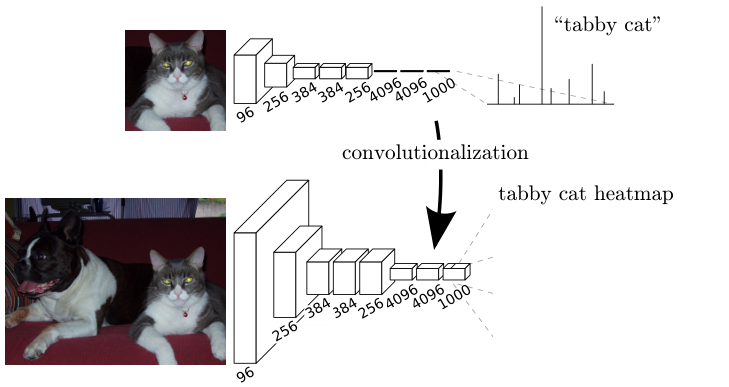
The upper part shows classification of one input; the lower part shows a spatial score map for a larger input. Do not confuse this classifier output with the later output of a 21-channel segmentation head for PASCAL. The figure first demonstrates that the spatial scope of computation can expand without changing the weights.
Jonathan Long, Evan Shelhamer, Trevor Darrell · 2015-03-08 · 1411.4038v2 original · Figure in the paper · Enlarge Excerpt from the original paper. Only the figure region was cropped and converted to lossless WebP; content and colors were not redrawn. Commentary was written separately and translated for this edition. Rights remain with the original rights holders; neither the blog code’s MIT license nor permission for CC redistribution is implied.Read the figure from input to output. Early convolutional layers extract features from small windows. Retaining output positions through the final layers allows each position to be traced to the input region it observes: its receptive field. Applying the same filters to a larger input does not mean feeding the entire larger image into a new fully connected layer. It means sharing the same local operations across more locations.
#What replacing a fully connected layer with convolution actually computes
A fully connected layer does not always become a 1×1 convolution. The kernel must cover the spatial extent originally seen by that layer. Consider flattening 7 × 7 × 512 features into 4,096 outputs. Each weight row reads 25,088 values. Reshaping it as one 7 × 7 × 512 kernel computes the same inner product; 4,096 rows become 4,096 output filters. A subsequent layer mixing channels at 1 × 1 × 4096 can be represented as a 1×1 convolution. The 7×7 example illustrates the conversion principle; it is not a definitive table of every intermediate tensor size with the actual FCN’s padding and cropping omitted. FCN v2, §3.1
The following explanatory reformulation expands the operation in indices. Assume stride 1, no padding, C input channels, and kernel size k. It uses the cross-correlation notation commonly called convolution in deep learning libraries.
o denotes the output channel, (i,j) the output’s spatial location, and (u,v) the position within the kernel. The first window computes the same inner product as a fully connected layer; moving the window computes the next location with the same weights. Because no new weights are created for each location, the same filters can process larger inputs. Inputs must still satisfy the network’s minimum-size, stride, and boundary-handling requirements.
A small numerical check: Where flattening and convolution coincide
Let the single-channel input be [[1, 2, 4], [3, 5, 8], [6, 9, 13]], the kernel [[1, 0], [0, -1]], and the bias 0. Flattening the upper-left 2×2 window gives [1, 2, 3, 5]. Its inner product with weights [1, 0, 0, -1] is 1 − 5 = −4. Applying the same computation to the right window gives 2 − 8 = −6; the lower-left gives 3 − 9 = −6, and the lower-right 5 − 13 = −8.
The output map is [[-4, -6], [-6, -8]]. Its first value is the fully connected output; collecting all four values gives the convolutional output. The image content has not changed: the same weights are being evaluated at more locations. This example verifies weight rearrangement; it is not an accuracy experiment from the paper.
Independent sliding-window classification can repeatedly compute regions shared by neighboring windows. FCN computes the common early feature map once and shares spatial operations in later layers as well. Running a new network for each pixel and computing all output locations with one network may pursue similar predictions, but their computational costs differ. The paper’s whole-image training discussion focuses on reducing this duplication in both forward and backward passes. FCN v2, §3–3.4
#Why does converting a classifier still leave coarse boundaries?
Retaining spatial information does not mean retaining it at the original pixel spacing. Accumulated pooling and strides separate neighboring final locations in input coordinates. The 32 in FCN-32s is the output stride of its coarse predictions, not the layer count or output side length. Upsampling the final score map by 32 cannot recover observations of boundaries already lost. FCN v2, §4.1–4.2
Separate two questions. “Is there a vehicle near here?” benefits from a broad receptive field. “Exactly which pixel marks the vehicle–background boundary?” needs fine localization. Deep features carry broad context at low resolution; shallow features are denser but cannot easily determine object semantics on their own. Discarding deep features and using only shallow ones does not solve the problem.
#Reading Figure 3 as a computation graph: 32s → 16s → 8s
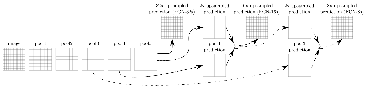
The upper single path is FCN-32s. The middle path incorporates pool4 scores; the lower path also incorporates pool3 scores. Intermediate convolutions omitted from the diagram still exist in the actual model. The grids must also be aligned to the input positions they represent.
Jonathan Long, Evan Shelhamer, Trevor Darrell · 2015-03-08 · 1411.4038v2 original · Figure in the paper · Enlarge Excerpt from the original paper. Only the figure region was cropped and converted to lossless WebP; content and colors were not redrawn. Commentary was written separately and translated for this edition. Rights remain with the original rights holders; neither the blog code’s MIT license nor permission for CC redistribution is implied.The paper does not add raw pool4 features directly to final class scores. It first projects them into class scores with a 1×1 convolution. Deep predictions have the same class channels. After aligning both outputs to the same spatial grid, it combines them by elementwise summation. FCN-8s adds pool3 class scores in the same way. This sum differs from the channel concatenation used later in U-Net. FCN v2, §4.2
The equations below are explanatory notation summarizing Figure 3, not numbered equations from the paper. S4 and S3 are pool4 and pool3 projected into class scores; U2 and U8 enlarge spatial dimensions. Align represents cropping and coordinate alignment to the target grid.
This is an illustrative size example assuming padding offsets have already been aligned. It does not transcribe actual intermediate Caffe model sizes. The batch dimension is omitted.
| Location | Example tensor size | Role |
|---|---|---|
| Deep class scores | 16×16×21 | Coarse semantic information at stride 32 |
| 2× upsampling + pool4 scores | 32×32×21 + 32×32×21 | Add matching class channels |
| 2× upsampling + pool3 scores | 64×64×21 + 64×64×21 | Add scores on a finer grid |
| Final 8× upsampling and alignment | 512×512×21 | Class scores for each output pixel |
Here, 21 is the PASCAL output-channel count including background. Adding two 32×32×21 tensors still yields 32×32×21. Concatenating them as in U-Net would yield 42 channels. Do not take argmax to obtain class IDs before addition. Adding class 3 to class 5 does not meaningfully produce class 8. Combine continuous scores first, then select the class at the end.
#How the loss trains the whole image
Summing losses across all valid output locations also sums their gradients. The following expands the discussion in §3 of the paper using cross-entropy. Ωvalid is the set of locations included in training. Implementation must specify how ambiguous labels are excluded and whether losses are summed or averaged.
This does not mean that running independent patch SGD in any order produces identical training. The relationship applies when gradients from the same samples at the same parameters are aggregated with the same normalization and update. Updating parameters after each patch or changing the sampling distribution can alter the optimization path. FCN’s advantage is reusing early computations across overlapping locations. FCN v2, §3.4
#What do the original results support?
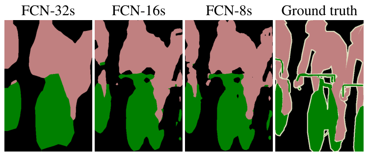
From left to right: 32s, 16s, 8s, and ground truth. These are segmentations from models combining different prediction strides, rather than simply enlarged photographs. This single qualitative example guarantees neither overall dataset performance nor improvements at every boundary.
Jonathan Long, Evan Shelhamer, Trevor Darrell · 2015-03-08 · 1411.4038v2 original · Figure in the paper · Enlarge Excerpt from the original paper. Only the figure region was cropped and converted to lossless WebP; content and colors were not redrawn. Commentary was written separately and translated for this edition. Rights remain with the original rights holders; neither the blog code’s MIT license nor permission for CC redistribution is implied.Read the numbers under matching conditions as well. The following mean IU results concern the VOC2011 validation subset in v2 Table 2. That subset excludes overlap with the additional training data; do not mix these figures with VOC2012 test results. FCN v2, Table 2 and §4.3
| Model | mean IU (%) | Question this comparison addresses |
|---|---|---|
| FCN-32s-fixed | 45.4 | Is fine-tuning only the final layer sufficient? |
| FCN-32s | 59.4 | What changes when all pretrained representations are adapted for segmentation? |
| FCN-16s | 62.4 | What is gained by incorporating finer pool4 scores? |
| FCN-8s | 62.7 | How much additional benefit remains after adding pool3? |
The rise from 59.4 to 62.4 is 3.0 percentage points; from 62.4 to 62.7, 0.3 points. This comparison alone does not establish that adding more skips always yields large gains. Nor should the difference between final-layer-only and whole-network fine-tuning be attributed to skips. Rankings assembled from incompatible data splits and training conditions change the meaning of the numbers.
Section 4.3 of v2 states that the final upsampling filter was fixed to bilinear interpolation, while intermediate upsampling filters were initialized bilinearly and learned. Saying either “all FCN upsampling is learned” or “all of it is fixed interpolation” misses this version’s actual setup. Later papers or public code may use different settings; verify their versions separately. FCN v2, §4.3
FCN’s central lesson is three connected ideas: reinterpret fully connected weights as spatial operations, combine coarse semantic scores with fine localization scores, and adapt the whole network through pixel-level losses. Saying only that it uses 1×1 convolutions does not explain these connections.
#6.2 What an encoder–decoder loses and recovers
The encoder expands its receptive field while reducing resolution through strides and pooling. This helps decide, in broad context, whether a pixel belongs to a car, but blurs precise boundaries. The decoder enlarges score maps using interpolation, unpooling, transposed convolution, or related operations.
The encoder compresses localization information to obtain broad context; the decoder restores spatial resolution using interpolation or transposed convolution.
When convolution is written as a linear operator, transposed convolution corresponds to its transposed matrix. One input can contribute to multiple output positions, but the operation is not an inverse that uniquely recovers lost inputs. Check output dimensions with the following relationship: s is stride, p padding, d dilation, k kernel size, and o output padding.
Worked example: Why transposed convolution is not a matrix inverse
Consider this one-dimensional valid operation. Kernel [1, 2] maps an input of length 3 to an output of length 2.
C is 2×3, and Cᵀ is 3×2. Increasing the length again does not restore the original values. This illustrates the meaning of transposition, not the specific numerical upsampling kernel used by FCN. Correct output dimensions and recovered information are different questions.
Uneven kernel overlap across positions can produce checkerboard artifacts. This is an implementation concern separate from the original papers’ numerical results here. Check grid alignment, interpolation, and boundary patterns as well as output dimensions.
#6.3 U-Net and skip connections
U-Net connects a contracting path and an expanding path. Recognizing the U shape alone misses half the original design: size reductions from valid convolutions, cropped feature concatenation, a boundary-weighted training objective, and augmentation of scarce annotated images all matter. The following describes the 2015 original; later variants with same padding, BatchNorm, or Dice loss are not presented as the original. U-Net v1, §2–3
Concatenate deep semantic information with shallow localization features to recover small objects and boundaries.
#Original Figure 1: What does each arrow change?
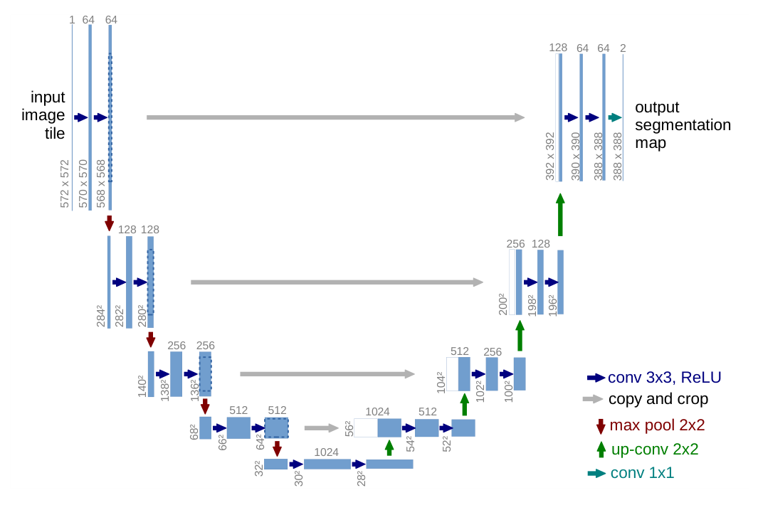
Blue boxes represent multi-channel feature maps. Numbers above give channel counts; numbers beside them give spatial dimensions. Downward red arrows are 2×2 max pooling, upward green arrows are 2×2 up-convolution, and gray arrows copy and crop encoder features. White portions on the right represent encoder features to be concatenated.
Olaf Ronneberger, Philipp Fischer, Thomas Brox · 2015-05-18 · 1505.04597v1 original · Figure in the paper · Enlarge Excerpt from the original paper. Only the figure region was cropped and converted to lossless WebP; content and colors were not redrawn. Commentary was written separately and translated for this edition. Rights remain with the original rights holders; neither the blog code’s MIT license nor permission for CC redistribution is implied.The left path applies two 3×3 convolutions and ReLU, then reduces spatial dimensions with 2×2 max pooling. Channel counts increase through 64, 128, 256, 512, and 1024. On the right, 2×2 up-convolution enlarges the spatial dimensions and reduces channels; corresponding left-path features are cropped and concatenated along channels. Two subsequent 3×3 convolutions process the combined information, and a final 1×1 convolution produces output class scores. U-Net v1, §2
Unlike a generic block diagram, the original figure labels dimensions after operations. Rather than stopping at “symmetric encoder–decoder,” follow the actual numbers beginning 572 → 570 → 568. Tracking how much the grid shrinks at each stage shows why cropping is necessary.
#Why does 572×572 become 388×388?
A 3×3 convolution without padding reduces each axis by 2 pixels; two reduce it by 4. Pooling and up-convolution introduce further changes. The following table arithmetically expands Figure 1’s operations. It lists one side length for square images and omits the batch dimension.
| Location | Spatial-size changes | Channels after two convolutions |
|---|---|---|
| encoder 1 | 572 → 570 → 568 → pooling 284 | 64 |
| encoder 2 | 284 → 282 → 280 → pooling 140 | 128 |
| encoder 3 | 140 → 138 → 136 → pooling 68 | 256 |
| encoder 4 | 68 → 66 → 64 → pooling 32 | 512 |
| bottleneck | 32 → 30 → 28 | 1024 |
| decoder 1 | up 56 → 54 → 52 | 512 |
| decoder 2 | up 104 → 102 → 100 | 256 |
| decoder 3 | up 200 → 198 → 196 | 128 |
| decoder 4 | up 392 → 390 → 388 | 64 |
| Output head | 388 → 388, 1×1 convolution | Number of predicted classes |
The original output is therefore smaller than the input: it predicts a central region using broader input context. The caption’s “lowest resolution 32×32” refers to the grid immediately after the final pooling operation. After the next two valid convolutions, the bottleneck feature in the figure is 28×28. U-Net v1, Figure 1
Worked example: Calculating crop sizes and concatenated channels
The first decoder-stage feature is 28×28×1024. Up-convolution makes it 56×56×512. The corresponding encoder feature is 64×64×512, so they cannot yet be concatenated. To retain the central 56×56 region, crop (64−56)/2 = 4 pixels from each side.
Concatenating two 56×56×512 tensors along channels produces 56×56×1024. The next two valid 3×3 convolutions reduce spatial dimensions to 56→54→52 and ultimately yield 512 output channels at this stage.
The same calculation applies to the remaining skips: crop 16 pixels per side for 136→104, 40 for 280→200, and 88 for 568→392. Skip crops of 4, 16, 40, and 88 differ from the 92-pixel input–output margin. The former align particular feature maps; the latter measures the valid-region difference between the network’s overall input and output.
The long gray arrows carry localization cues that the decoder must recover. This does not mean every encoder activation already represents an exact boundary. Subsequent convolutions must learn to combine deep context and shallow features. Having a skip connection alone guarantees no boundary accuracy.
#Distinguishing FCN skips from U-Net skips
Both models link shallow and deep layers, but differ in what they combine and how they combine it.
| Comparison | FCN-16s/8s | Original U-Net |
|---|---|---|
| What shallow layers supply | Outputs projected into class scores | Multi-channel encoder features |
| Combination | Sum scores at matching locations and classes | Concatenate cropped features along channels |
| Channels immediately afterward | Class count unchanged | Sum of the two input channel counts |
| Subsequent role | Form predictions on a finer grid | Reprocess combined features with convolutions |
This table compares the two original architectures; it is not a performance ranking under identical conditions. FCN v2, §4.2, U-Net v1, §2
Writing encoder features as E and decoder features as D, the U-Net combination is as follows. ConvBlock does not mean simple addition; it groups operations such as the two learned convolutions.
Even “join tensors of the same size” needs care. The original encoder features are larger; their sizes match after cropping. Adding padding to preserve size may be useful, but mixing that variant with the original tensor trace will not reproduce 572→388.
#U-Net’s original loss: Spatially weighted cross-entropy, not Dice
The paper applies softmax to each pixel’s class scores and combines it with a spatial weight map. Writing the logit for class k at pixel x as a_k(x) gives the following probability. Softmax sums over classes at the same pixel, not across pixels. U-Net v1, §3
ℓ(x) is the ground-truth class, Ω the evaluated output-pixel region, and w(x) the spatial weight multiplying the training loss. Equation (1) in v1 is written without a minus sign, as below. Its original notation is preserved.
To use this as a negative log-likelihood loss to minimize in code, define the following separately. The minus sign below clarifies the minimization objective; it is not a verbatim transcription of the original equation.
As the correct-class probability rises from 0.1 to 0.9, log p increases from approximately −2.303 to −0.105. Conversely, −log p decreases from 2.303 to 0.105. Calling the original E a cross-entropy to minimize would therefore conflict with its sign. This numerical check helps catch a common transcription error.
The Dice-family objectives introduced later in §6.5 are additional comparisons of segmentation losses. Do not read this as saying that the 2015 U-Net was trained with Dice loss. Its distinctive training device is the boundary weight map below.
#Original equation (2): Why penalize the gap between touching cells more heavily?
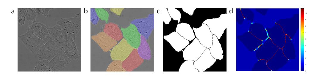
Panel (a) is the original image, (b) the instance-labeled ground truth, (c) the training segmentation mask, and (d) the loss weight map. Look at the narrow gaps between touching cells. Panel (d) is prepared from ground truth for training; it is neither a predicted probability map nor an attention map.
Olaf Ronneberger, Philipp Fischer, Thomas Brox · 2015-05-18 · 1505.04597v1 original · Figure in the paper · Enlarge Excerpt from the original paper. Only the figure region was cropped and converted to lossless WebP; content and colors were not redrawn. Commentary was written separately and translated for this edition. Rights remain with the original rights holders; neither the blog code’s MIT license nor permission for CC redistribution is implied.If most pixels are foreground, correctly classifying cell interiors can greatly reduce average loss. Yet filling the thin background gap between two cells makes them appear merged. The affected area is small, but the interpretation matters. Beyond class-frequency correction, U-Net adds a term emphasizing these separating boundaries between cells. U-Net v1, Figure 3 and equation (2)
w_c(x) corrects class-frequency imbalance. d1(x) is the distance to the nearest cell boundary; d2(x) the distance to the second-nearest cell boundary. These are neither errors between predicted and true masks nor merely distances to the outer image border. w0 controls the additional weight, and σ its distance-dependent decay. The paper’s experiments use w0=10 and σ≈5 pixels.
Read the exponent rather than memorizing left to right. Near both cell boundaries, d1+d2 is small, so the negative exponent has smaller magnitude and the added term is larger. Near one boundary but far from another cell, the distance sum grows and the extra term shrinks. Thus the term does not assign the same high weight to every outer boundary. The numerator is (d1+d2)², not d1²+d2².
Worked example: How boundary weights change the probability gradient
For illustration, fix wc=1, w0=10, and σ=5. With distances d1=1, d2=1, the first pixel’s weight is approximately 10.2312. With d1=1, d2=9, the second pixel’s weight is about 2.3534. Both lie one pixel from the nearest boundary, but the second-nearest boundary changes their penalties. wc=1 is chosen for this example, not claimed as the class weight of the paper’s entire dataset.
If both pixels assign probability 0.5 to the correct class, their losses are wA×log 2 and wB×log 2. The first pixel contributes about 4.35 times as much despite the same probability error. The following gradient is an explanatory differentiation of weighted softmax cross-entropy, not a numbered equation from the paper. The target indicator is y_k(x).
In the correct-class channel, when p=0.5, y=1 the gradient is −0.5w. Larger boundary weights send stronger parameter-update signals for the same error. The map is prepared from ground truth; this does not describe learning w itself as an attention parameter. Averaging the loss also multiplies the entire gradient by the chosen normalization constant.
Remember that distances are measured in pixels. After halving image dimensions, emphasizing a boundary of the same physical width requires reconsidering the relation between distances and σ. This is an arithmetic consideration when resizing images, not a new experimental result. The weight map is not a ground-truth input channel supplied at inference, which also matters when checking for data leakage.
#Handling large images: Overlap tiles and mirrored context
Predicting a central region does not restrict the original model to processing only 388×388 images. Larger images can be divided into input tiles whose valid output regions are stitched together. The paper describes overlap-tile inference, using mirroring to provide context at image edges. U-Net v1, Figure 2
For the 572-input/388-output diagram, the symmetric margin is (572−388)/2=92. Spacing output tiles by 388 makes input tiles overlap by 572−388=184. These numbers are worked calculations for Figure 1. Overlapping input tiles with adjacent usable central outputs lets the model read broad context while avoiding incomplete predictions near tile edges.
Mirroring context at the input image boundary differs from adding same padding to every convolution. The former supplies context outside a tile; the latter preserves feature dimensions within network layers. Cropping encoder features to decoder dimensions is another step again. Calling all three “padding” obscures output-alignment checks.
#Other training devices for scarce annotated data
The paper emphasizes strong data augmentation, especially elastic deformation: generate random displacements on a small grid and interpolate a smooth deformation field. It specifies a coarse 3×3 grid, Gaussian displacement standard deviation of 10 pixels, and bicubic interpolation. Large input tiles, batch size 1, and momentum 0.99 are also part of its training setup. U-Net v1, §3–3.1
The aim goes beyond making many copies of a small collection. Slightly stretching or bending cells while retaining their labels supplies deformation invariance. Augmentation nevertheless does not create new independent experimental subjects or hospital datasets. Variants share original images, so evaluation splits and independence must be maintained separately.
Implementation note: Keep the original design distinct from modern choices
The following is a reproduction checklist, not a verbatim list of paper settings. Apply the same coordinate field to images and labels during geometric transforms. Interpolating class-ID masks as continuous values can invent labels, so specify label interpolation separately. Some loss APIs take logits rather than probabilities; check for duplicate softmax. Exclude ignored labels consistently from both weighting and reduction.
Same padding, BatchNorm, pretrained encoders, combined Dice/cross-entropy losses, and 3D convolution are separate design choices. They may be useful, but labeling such a model an identical reproduction of the 2015 original requires stating the changes. Attaching a 572×572 target directly to the original 572→388 architecture already breaks the loss’s spatial correspondence.
#What was tested, and how far do the conclusions extend?
The cell and electron-microscopy tasks are not the same benchmark as PASCAL natural-image segmentation. Reported segmentation IoUs for PhC-U373 and DIC-HeLa are 0.9203 and 0.7756, respectively. Placing these alongside FCN’s 21-class mean IU cannot establish that U-Net is universally better: datasets, labels, metrics, and evaluation procedures differ. U-Net v1, §4
The electron-microscopy task’s 30 annotated images do not mean 30 independent patients. The paper describes serial-section electron microscopy of the Drosophila nervous system. Results with scarce annotations matter, but do not guarantee performance across all medical images or clinical deployments. Using the same architecture for three tasks also does not mean a single checkpoint solved all three simultaneously.
Figure 3’s ground truth distinguishes individual cells, but semantic classes and instance IDs must remain distinct when describing the final model output. Learning background gaps can help separate instances later; it does not automatically make U-Net’s output head predict unique instance IDs. Read the failure targeted by the weighting together with the final task definition.
U-Net is more than an encoder–decoder with skips. Understanding its architecture and training means tracing resolution changes, checking concatenated channels, calculating which gradients ground-truth boundary weights amplify, and distinguishing augmentation from evaluation scope.
#6.4 Enlarging context with dilation while retaining resolution
FCN and U-Net ask how to combine coarse semantics with precise localization. Add another question: How can we gather context at different scales without continually reducing resolution? PSPNet pooling grids and DeepLab dilation rates both address multiple scales, but are different operations. This section uses the architectures and comparative experiments of PSPNet 1612.01105v2, DeepLabv3 1706.05587v3, and DeepLabv3+ 1802.02611v3.
Apply kernels with different sampling intervals in parallel without further reducing feature-map resolution. DeepLab ASPP combines these responses into multiscale context.
#PSPNet: Reading the whole scene and its regions together
When local patch shape is ambiguous, the surrounding scene offers clues. But pooling every location into one global vector loses distinctions between regions. PSPNet retains the original features while appending summaries of the whole scene, large regions, and smaller regions. Its central device is the pyramid pooling module, or PPM. PSPNet, §3.2–3.3, Figure 3
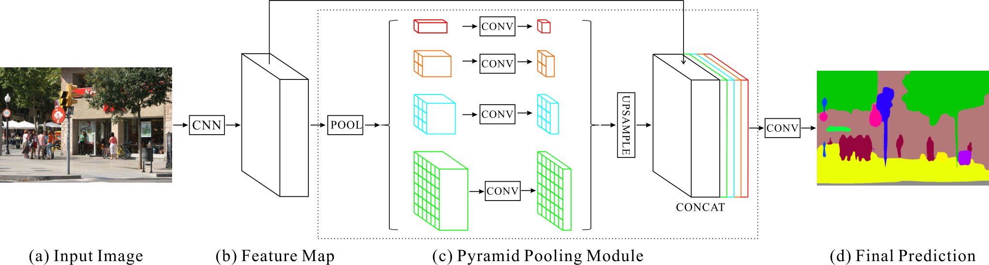
Starting from the left CNN output, follow the four paths inside the dashed box. Colors mark different pooling grids. CONV processes each small grid; its output is enlarged to the original spatial size, then concatenated with the initial features. The final segmentation is learned from this combination, not obtained by directly coloring pooling values.
Hengshuang Zhao et al. · 1612.01105v2 · Original paper · Figure in original · Enlarge Excerpt from the original paper. The original PNG is used unchanged. Commentary was written separately and translated for this edition. Rights remain with the original rights holders; the blog code’s MIT license does not grant figure redistribution rights.Here, 1, 2, 3, 6 denotes the number of output bins along one side after pooling. It does not mean applying 1×1/2×2/3×3/6×6 convolutions, nor dilation rates 1/2/3/6. A 1×1 grid summarizes the whole image; 2×2 distinguishes four large regions. Finer grids summarize smaller regions.
The following reformulates Figure 3 using explanatory operator notation, not original equation numbers. F is the encoder feature, A_b average pooling to b×b outputs, φ_b a learned operation such as a 1×1 channel transform, and U bilinear resizing.
Worked example — a 60×60×2048 feature tensor. The size 60 avoids rounding. This is illustrative, not a claim that all paper images produce 60×60 intermediate features. With four branches reduced to 512 channels each, the following holds.
| Path | H×W×C after pooling | After channel reduction | After resizing |
|---|---|---|---|
| global | 1×1×2048 | 1×1×512 | 60×60×512 |
| 2-grid | 2×2×2048 | 2×2×512 | 60×60×512 |
| 3-grid | 3×3×2048 | 3×3×512 | 60×60×512 |
| 6-grid | 6×6×2048 | 6×6×512 | 60×60×512 |
Including the original 2048 channels yields 60×60×4096. Since 2048+4×512=4096, summing the four pooled outputs would not reproduce this channel count. Only in this example does each bin of the 6-grid average a 10×10 region. When dimensions do not divide evenly by the grid, check adaptive-pooling interval assignment and implementation.
Upsampling a global 1×1 value to 60×60 supplies the same global information everywhere. Grids of 2×2 or more can supply position-dependent context. Resizing does not observe fine boundaries lost during summarization. The original features therefore remain in the concatenation: context summaries and localization serve different roles.
Training also uses an intermediate auxiliary classification loss. The following summarizes the objective using 0.4, one of the auxiliary-loss weights studied in the paper. The auxiliary head need not run as a second final predictor during inference. PSPNet, §4, Table 2
What did the experiment establish? The following is the ADE20K validation, ResNet-50, single-scale comparison in Table 1. Its baseline uses that section’s training setup; do not mix in a weaker baseline from elsewhere. These are the paper’s mean IoU values, not independently reproduced results.
| Configuration within Table 1 | mIoU (%) |
|---|---|
| baseline | 37.23 |
| Add global average pooling only | 40.07 |
| Average pooling at four grids | 41.07 |
| Four grids + average pooling + dimension reduction | 41.68 |
37.23→41.68 is 4.45 percentage points; the gain over global-only is 1.61 points. This supports multiregion context under these conditions, not a universal gain from one pooling operation. Subtracting scores with different auxiliary losses, augmentation, backbones, or multiscale testing cannot isolate PPM’s contribution. PSPNet Table 1, single-scale/multiscale results in the authors’ implementation
#DeepLabv3: Changing convolutional sampling intervals rather than pooling regions
Atrous convolution changes sampling intervals without adding filter coefficients. Its one-dimensional form is below: r is the dilation rate, and w[k] the learned coefficients. The same principle applies along both axes in two dimensions. DeepLabv3, §3, equation (1)
Worked example. A 3×3 kernel with r=6 spans 13 positions along each axis. It still learns only 9 spatial coefficients, rather than a dense 13×13 kernel reading all 169 positions. No newly learned coefficients are inserted between taps. Samples spread farther apart, but this layer does not observe every intervening position.
Dilation alone does not automatically preserve resolution. The following is the general operator formula for one-dimensional output size.
For k=3, r=6, s=1 to preserve input size under this symmetric-padding example, p=6 is required. With p=0, size shrinks to H−12. Specify receptive field, stride, dilation, and padding separately. Some boundary samples read padding rather than actual image values.
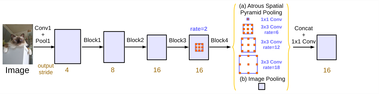
The ASPP module on the right has five branches: a 1×1 path, three paths with rates 6/12/18, and an Image Pooling path. Backbone stride and within-block multi-grid settings are distinct from these parallel branches.
Liang-Chieh Chen et al. · 1706.05587v3 · Original paper · Figure in original · Enlarge Excerpt from the original paper. The original PNG is used unchanged. Commentary was written separately and translated for this edition. Rights remain with the original rights holders; the blog code’s MIT license does not grant figure redistribution rights.At output stride 16, the improved DeepLabv3 ASPP combines one 1×1 branch, three 3×3 atrous branches, and image-level pooling. Each has 256 channels; a post-concatenation 1×1 transform returns the result to 256 channels. DeepLabv3, §3.2, Figure 5
Worked example — a 32×32 encoder feature. The four convolution branches each produce 32×32×256. The global-pooling branch transforms channels at 1×1, then resizes to 32×32×256. Concatenation gives 32×32×1280, and projection gives 32×32×256. Unlike PSPNet’s four pooling grids, ASPP’s atrous branches sample the same spatial grid at different intervals.
For the same input, lowering output stride from 16 to 8 ideally doubles each feature dimension, quadrupling the number of positions. Doubling r maintains roughly the same spacing in input coordinates; the paper’s OS=8 inference uses 12/24/36. Actual shapes for odd input sizes depend on padding and rounding: a noninteger such as 513/16 does not specify an exact feature shape.
Larger rates are not always better. When samples spread too far relative to the feature map, many fall outside its boundary. In the extreme, only the center tap remains valid, undermining the intended broad context. Image pooling supplies a separate global-summary path instead of merely increasing one dilation rate.
Changing modules under matched conditions. In Table 5, ResNet-101 on VOC validation at output stride 16 with Multi-grid (1,2,4) + ASPP(6,12,18) achieves 76.58%. Adding rate 24 gives 76.46%; adding image pooling yields 77.21%. More paths do not improve performance monotonically; the image-level path adds 0.63 points in this comparison. DeepLabv3, Table 5
The sequence 77.21→78.51→79.45→79.77→82.70 in Table 6 changes evaluation output stride, multiscale inference, flipping, and COCO pretraining successively. Do not attribute the entire final-minus-initial gain to ASPP. Learned-module effects differ from the effects of more expensive inference and additional training data.
#DeepLabv3+: Adding a decoder to refine boundaries after gathering context
DeepLabv3+ asks whether gathering context with ASPP is sufficient. Rather than enlarging coarse high-level features in one step, it combines them with denser low-level features and refines them spatially. It shares U-Net’s encoder–decoder goal, but not the original U-Net’s repeated connections at every resolution level. DeepLabv3+, §3, Figure 2
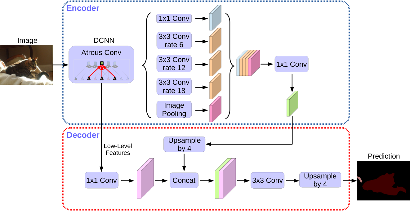
The encoder is above and the decoder below. Features, not class IDs, enter the decoder. Follow the order: the low-level feature’s 1×1 transform and the upper feature’s fourfold upsampling both precede CONCAT.
Liang-Chieh Chen et al. · 1802.02611v3 · Original paper · Figure in original · Enlarge Excerpt from the original paper. The original PNG is used unchanged. Commentary was written separately and translated for this edition. Rights remain with the original rights holders; the blog code’s MIT license does not grant figure redistribution rights.Worked example — an aligned grid for a 512×512 input with encoder OS=16. This illustrates the operations; it does not replace the paper’s odd crop sizes or actual shape tables for every backbone.
| Location | Tensor H×W×C | Purpose |
|---|---|---|
| Encoder output | 32×32×256 | Features carrying ASPP context |
| 4× bilinear upsampling | 128×128×256 | Spatial alignment with the low-level grid |
| 1×1 low-level projection | 128×128×48 | Reduce shallow-feature channels |
| Channel concatenation | 128×128×304 | 256+48, not a score sum |
| Two 3×3 refinement operations | 128×128×256 | Process combined context and localization |
| Class head and final resize | 512×512×K | Per-pixel logits |
The 48 channels are not the original low-level feature’s channel count; they are the output of the channel projection. This is an experimentally examined design choice, not a uniquely optimal constant across arbitrary datasets and backbones. Likewise, increasing refinement from two 3×3 convolutions to three did not automatically improve results. DeepLabv3+, Tables 1–2
#Where atrous separable convolution saves computation
Separate spatial depthwise convolution, performed independently per channel, from pointwise 1×1 convolution, which mixes channels. Dilation applies at the spatial sampling stage. The following calculation assumes multiplier=1 and excludes biases and normalization parameters.
With k=3 and 256 input/output channels, ordinary convolution has 589824 parameters; separable convolution has 67840. The approximately 8.69-fold difference is not a measured 8.69-fold speedup on real hardware. Memory traffic, intermediate tensors, kernel launches, and hardware support also matter. Nor can an arbitrary dense convolution always be replaced losslessly by the same depthwise–pointwise filters: the representational structure changes.
Reading accuracy and computation together. The following uses matched conditions from Table 3: VOC2012 validation, ResNet-101, training/evaluation OS=16, single scale, and no flipping. B denotes billions; the source column is named Multiply-Adds.
| Configuration | mIoU (%) | Multiply-Adds |
|---|---|---|
| Without decoder | 77.21 | 81.02B |
| With decoder | 78.85 | 101.28B |
Under these conditions, adding the decoder gains 1.64 points while adding 20.26B operations. “Lightweight decoder” does not mean zero cost. Do not mix this ResNet comparison with best scores using Xception, extra data, or multiscale evaluation to estimate the decoder’s isolated effect. DeepLabv3+, Table 3, PDF p.9
#Questions that distinguish the three architectures
For PSPNet, ask which regions are summarized. For DeepLabv3, ask at what intervals spatial samples are read and how global summaries are added. For DeepLabv3+, ask which low-level features join the contextual features to refine boundaries. Pooling grids, dilation rates, and decoder roles matter more than a pyramid-like appearance. Record channel axes, bilinear-resize coordinate settings, training/evaluation output strides, BN training conditions, and original label resolution.
#6.5 Pixelwise losses and class imbalance
The most direct objective sums cross-entropy across pixels.
Large classes such as sky and road can occupy far more pixels than small signs or pedestrians, causing average loss to favor large classes. Class weights can amplify errors on rare classes.
The original U-Net equation (2) adds spatial weights based on distances between cell boundaries, beyond class-frequency correction. A constant per class differs from a weight varying by pixel location.
Dice-family objectives directly measure overlap between predicted and target regions. The following is a general loss comparison, not the original U-Net training loss. It may be useful for small foreground regions, but batch composition and smoothing ε must also be specified.
Pixelwise probability errors in cross-entropy differ from region overlap in Dice. Using cross-entropy alone also does not guarantee calibrated probabilities. Distinguish the optimized objective from evaluation of per-class IoU, boundary quality, and probability reliability.
#6.6 MRFs: Adding spatial structure after prediction
First distinguish the names. A Markov random field (MRF) models spatial dependencies; ICM optimizes labels in a specified model. An MRF is not a type of CNN, and ICM need not train a neural network. This section uses Besag’s 1986 paper as historical context, while directly verifying calculations in a separately defined small Potts model. Besag, On the Statistical Analysis of Dirty Pictures, JRSS B 48(3), 1986
In the existing Gibbs equation, x is the state variable. To avoid ambiguity, the example below uses y for labels and x for observations, with temperature T=1. Keep source notation distinct from example notation.
Combine each pixel’s observation-fit cost with neighboring-label smoothness costs. ICM updates one location at a time to the label with the lowest local energy.
#What do the nodes and edges represent?
The conceptual diagram above is an existing explanatory illustration of updating neighboring labels one at a time, not a reproduced paper figure. It is not assigned a figure number suggesting verification of a particular original plate. Below, use a three-node chain 1—2—3. Nodes represent pixel or regional labels; edges represent a modeling choice to penalize label combinations. An edge does not mean the pixels have identical RGB values.
A four-neighbor image graph typically uses up, down, left, and right neighbors. An eight-neighbor graph including diagonals is possible but different. Changing the graph changes the energy and potentially its optimum; “we applied an MRF” is insufficient for reproduction. MRFs need not use only pairwise potentials; larger cliques are possible.
When invoking Hammersley–Clifford, check assumptions such as strict positivity in the appropriate finite-graph setting. Saying “only neighbors matter” does not establish equivalence between arbitrary distributions and arbitrary energy representations. All states in this example have finite energy, so the Gibbs distribution below assigns positive probabilities.
#Separating unary and pairwise costs numerically
Writing observations as x and labels as y, define the following conditional energy model. This is an explanatory model for this section, not a transcription of an original equation. Z normalizes probabilities over all label configurations to sum to 1.
Choose a Potts pairwise cost for a concrete example.
D_i(k;x) is the unary cost of assigning label k at position i; λ penalizes a label differing from its neighbor. Count each undirected edge once. Counting both i→j and j→i unintentionally doubles the pairwise weight. With λ=0, optimization separates into independent unary minimizations. Large λ favors equal labels but can erase thin real structures.
A Gaussian observation model can yield unary costs such as (x_i−μ_k)²/(2σ²). Alternatively, choose −log p_θ(k|X) from CNN probabilities. The latter is a conditional energy depending on the full observation X; without further assumptions, it is not the same as a purely generative p(x_i|y_i). The local Markov property concerns conditional independence among labels; it does not require unary costs to inspect only a small RGB patch.
#Why ICM need not search every complete labeling at each update
Holding all labels except i fixed makes energy terms unrelated to i constant. Remove those terms and compare only the unary term and edges involving i. The sequential update in this pairwise example is as follows.
Neighbors y_j use their most recently updated states. Maximizing conditional probability and minimizing the corresponding negative-log local energy choose the same label. Thus neither Z nor distant-node costs need be computed. This differs from applying independent unary argmins to all nodes simultaneously.
The following is a direct implementation for small label sets and neighborhoods. One sweep visits each node once. Retain the current label on ties to avoid meaningless cycles.
Choose initial labels y.
Visit each node i in the specified order.
    Compute local energy for every candidate label.
    Change the label only when its cost is strictly lower than the current label’s.
Stop when no labels change during a sweep.
If each change strictly decreases total energy and the state space is finite, the procedure terminates. But the result is a coordinatewise minimum that no single-node change improves, not necessarily a global optimum or posterior mean. Record floating-point tolerances, node order, initialization, maximum sweeps, and whether convergence actually occurred.
#Worked example 1: Why isolated noise can disappear
Use graph 1—2—3, labels 0/1, and λ=0.6. Define the unary costs below. These numbers illustrate the operation; they are not estimates from data.
| Node | D(0) | D(1) | Unary-only choice |
|---|---|---|---|
| 1 | 2.0 | 0.0 | 1 |
| 2 | 0.0 | 0.4 | 0 |
| 3 | 2.0 | 0.0 | 1 |
The initial 101 has unary sum 0 and two disagreeing edges, for total cost 1.2. Keeping the center at 0 gives local cost 1.2; changing it to 1 gives 0.4+0=0.4. Updating the center therefore yields 111 with total cost 0.4. This is one way spatial consistency can remove an isolated prediction.
If the center is genuinely a small object, changing it need not be correct. The model merely follows the chosen prior that disagreement with neighbors incurs cost. Lower energy and higher real segmentation accuracy require separate verification.
#Worked example 2: ICM can stall despite a better global solution
For two nodes 1—2, assign D(0)=1 and D(1)=0 to each, with λ=2. Enumerate every possible state.
| State | Unary sum | Pairwise cost | Total energy |
|---|---|---|---|
| 00 | 2 | 0 | 2 |
| 01 | 1 | 2 | 3 |
| 10 | 1 | 2 | 3 |
| 11 | 0 | 0 | 0 |
At 00, changing either node alone worsens cost from 2 to 3, so ICM stops. Yet 11 has cost 0. Changing both together helps, but changing one first incurs a penalty. These four states refute the claim that enough iterations always reach the global optimum. Random restarts try alternative starting points; finitely many do not generally guarantee global optimality.
#Worked example 3: Why parallel updates can break monotonic decrease
On the same two-node graph, set all unary costs to 0 and λ=1, starting at 01. If both nodes update simultaneously using only the previous sweep’s neighbors, the first chooses 1 and the second 0, producing 10; the next update returns to 01. Each matches its old neighbor, yet they remain misaligned. Immediate sequential updates instead reach 11 or 00.
This counterexample cautions against assuming that updating all GPU pixels in parallel equals original ICM. Checkerboard updates that partition nodes into independent sets with no within-group edges can be analyzed separately. Simple simultaneous and sequential updates should not share a name without distinguishing their behavior.
#What the original paper and these examples each support
Besag’s paper studies noisy-image restoration through probabilistic models and iterative local optimization. Here, publicly available bibliographic information and the abstract establish context; this is not a claim to have checked every original plate and restoration result. The three examples above are independently defined, exhaustively checked small models, not tables from the paper. Do not cite them as its measured restoration rates.
Even when adding spatial costs after a modern network, specify unary definitions, graph, λ, initialization, and update rules first. Do not interchange MRF and CRF solely by name, or claim DeepLabv3/v3+ necessarily retain older DeepLab’s DenseCRF postprocessing. Learned decoders and energy-based postprocessing incorporate spatial structure differently.
#6.7 What should be measured?
Pixel accuracy can overrate a model that predicts the background well. Per-class Intersection over Union (IoU) is the intersection of prediction and ground truth divided by their union.
Distinguish per-class IoU and its mean mIoU, recall for small classes, and boundary metrics. Check whether resizing and padding were reversed before evaluation: a one-pixel alignment error can strongly affect thin structures. For an original U-Net’s central valid output, targets must cover exactly the same positions.
Check your understanding: Suppose an image is 95% background and 5% foreground, and every pixel is predicted as background. Pixel accuracy is 95%, but foreground IoU is 0. The numbers show why high accuracy does not demonstrate good boundary recovery. This is an illustrative example, not a dataset ratio or result from the papers above.
#6.8 Connecting the pieces
The encoder builds broad context; the decoder restores spatial outputs. FCN skips add class scores, whereas U-Net skips concatenate features. Original U-Net valid convolutions shrink features, requiring crop and valid-output calculations. In losses, distinguish probability errors, class frequencies, and boundary importance. In evaluation, verify data, labels, splits, and alignment as well as metric names.
After reading, try explaining: When does a fully connected layer become 7×7 versus 1×1 convolution? Why does adding FCN scores leave channel counts unchanged? How are U-Net’s 572→388 trace and 4/16/40/88 crops calculated? How does the original E’s sign differ from a loss to minimize? Why can equal nearest-boundary distances yield different weights because of the second boundary?
FCN connected spatial dense-prediction computation with transfer learning. U-Net jointly designed feature fusion, valid output regions, and boundary-weighted training for biomedical localization. DeepLab dilation and spatial pyramids provide another axis for extending context. When reading a new architecture, ask what is computed at each resolution, what is combined, and which errors are penalized: operations then become clearer than names.
#Revisit the original papers and figures
Long, Shelhamer, and Darrell, FCN 1411.4038v2, 2015-03-08 — read Figure 2’s classifier conversion, Figure 3’s skip computation graph, and the comparisons in Figure 4 and Table 2 together.
Ronneberger, Fischer, and Brox, U-Net 1505.04597v1, 2015-05-18 — read Figure 1’s dimensions/channels, Figure 2’s overlap tiles, and Figure 3 with equations (1) and (2) together.
U-Net authors’ project page — a starting point connecting the paper with author-provided software. When using code or later models, verify versions and changes from the original separately.