Image denoising and generative modeling both relate observations to latent clean signals, but they are different tasks. Distinguish what is estimated, which distribution is learned, and whether information available during training is also available at inference. Existing lecture equations are retained, with original-paper evidence and separate worked examples added. Small numbers and tensor sizes in these examples are not reproduced paper experiments.
#7.1 Denoising as estimation
Suppose noise corrupts a clean value x to produce observation y. MSE evaluates a restorer through squared error between prediction and target. The decision minimizing squared error can differ from the decision to sample from the original distribution.
Linear MMSE uses a weighted sum over a neighboring patch; a median filter chooses a value minimizing absolute deviations within its window.
For the linear coefficient formula Rzz⁻¹rzx, check invertibility and whether variables are centered. A bias-free linear estimator differs from an affine estimator on nonzero-mean data. Numerically, solve the linear system rather than explicitly forming an inverse, and specify treatment of singular or ill-conditioned cases. These mathematical conditions explain how to apply the source’s compact equation.
Worked example. After observing y, suppose x equals −1 or +1 with probability 1/2 each. A constant prediction a has the following conditional squared error.
The minimum is a=0, although clean x never equals 0 in this example. The conditional mean being optimal for squared error does not require every generated sample to equal that mean. Averaging alternative image details can likewise produce blur, but this example does not explain every restorer’s blur.
#7.2 Why medians resist impulse noise
Worked example. For window values [10, 11, 12, 13, 255], the mean is 60.2 and the median 12. Unlike the mean, which the single value 255 pulls upward, the median depends on order. A median minimizes summed absolute deviations, but need not be unique: for the even-sized sample [0, 2], every value between 0 and 2 gives the same sum.
A restoration metric specifies which errors matter. In PSNR, L is the peak dynamic range used for the comparison. Interpret the following equation for MSE>0.
For L=1, MSE=0.01 gives 20 dB; MSE=0.0025 gives approximately 26.0206 dB. Quartering squared error gains about 6.0206 dB. Mixing 0–255 and 0–1 images while changing only L or MSE units produces invalid scores. The ideal MSE=0 case gives infinity; document any small constant used instead. PSNR alone cannot assess all texture realism or downstream detection performance.
#7.3 Discriminative and generative models
A classifier’s p(y|x) and a generator’s p(x) serve different purposes. A latent-variable model samples z from a prior, then generates x through pθ(x|z). Inferring z from observed x instead concerns posterior pθ(z|x). Below, encoder means qφ, which constructs an approximate posterior; decoder means pθ(x|z), which constructs the likelihood.
A stochastic decoder’s outputs differ from a deterministic value interpreted as the target image itself. A Bernoulli likelihood outputs pixel probabilities; a Gaussian likelihood outputs means and a chosen variance structure. Connect BCE or MSE reconstruction losses to this observation model. Kingma and Welling, Auto-Encoding Variational Bayes, §2–3
#7.4 VAE: Learning a tractable posterior approximation
The VAE problem is more specific than adding noise to a latent. A complex decoder makes pθ(x)=∫pθ(x,z)dz hard to compute, and this value also appears in the posterior denominator. Instead of repeating expensive inference for every x, train a neural-network approximation qφ(z|x). The paper first appeared in 2013; the linked text is v11, revised 2022-12-10. Distinguish the original release from the consulted version.
The encoder produces the mean and variance of qφ(z|x); reparameterization samples z, and the decoder reconstructs through pθ(x|z).
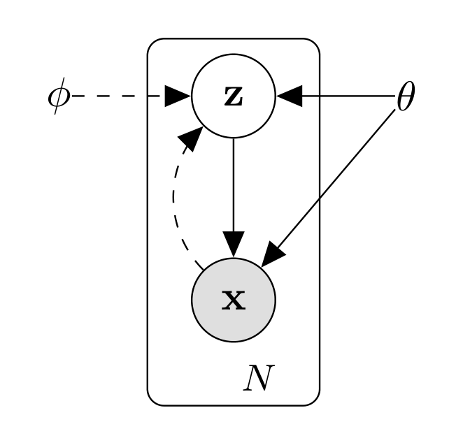
Do not reverse the solid generative and dashed inference directions. θ and φ are different parameter groups, not two names for one variable. N marks the plate repeating latent variables over observations. This is not a layer-by-layer convolutional encoder or U-Net diagram.
Diederik P. Kingma; Max Welling · 1312.6114v11 · Original paper · Figure in original · Enlarge Excerpt from the original paper. The figure region was cropped from the original PDF and rendered at high resolution. Commentary was written separately and translated for this edition. Rights remain with the original rights holders; the blog code’s MIT license does not grant figure redistribution rights.#Distinguishing the two KL divergences in the ELBO
The following restates the relations in original equations (1)–(3). The first KL measures the gap between the approximate and true posteriors; the second measures the gap between the approximate posterior and the prior.
Their right-hand distributions differ. ELBO is not used because the first KL can be evaluated directly. Since the true posterior is difficult, optimize the tractable lower bound on the second line. At fixed θ, increasing ELBO narrows the posterior-approximation gap; joint training of θ does not guarantee true likelihood increases monotonically at every minibatch.
Derivation. Substitute log pθ(x,z)=log pθ(z|x)+log pθ(x) into Eq[log pθ(x,z)−log q]. Since log pθ(x) does not depend on z, it leaves the expectation; the remaining Eq[log q−log posterior] is KL. Nonnegativity gives the lower bound. Turning maximization into an optimizer’s minimization loss changes the sign to −ELBO = reconstruction NLL + KL.
#Calculating Gaussian KL numerically
A standard-normal prior and diagonal Gaussian posterior give the following closed form. μ and σ are latent means and standard deviations; σ² is variance. AEVB, Appendix B
Worked example. For one latent dimension with μ=1 and σ=0.5, KL is 0.818147… nats. Substitute σ²=0.25. Conversely, μ=0 and σ=1 match the prior and give KL=0. If an implementation outputs logvar, then σ=exp(logvar/2), not exp(logvar).
Trace tensors in a small explanatory model: MNIST-like inputs with latent size 20. This table does not claim to represent every experiment in the paper.
| Value | Shape | Role |
|---|---|---|
| Input x | B×784 | Flattened 28×28 observation |
| μ, logvar | B×20 each | Posterior parameters, not samples |
| ε and z | B×20 each | External noise and reparameterized sample |
| Decoder logits | B×784 | Per-pixel logits for a Bernoulli likelihood |
| Reconstruction NLL, KL | B each | Per-sample sums over feature/latent axes |
| Final loss | Scalar | Chosen batch reduction |
Averaging over 784 pixels while summing 20 KL dimensions weights the terms differently from summing both per sample and then averaging the batch. Check whether a smaller loss reflects improvement or merely a changed reduction.
#Reparameterization does not eliminate sampling
Sample ε from a standard normal independent of θ and φ. Holding ε fixed expresses z as a differentiable function of μ and σ, letting the chain rule carry decoder loss through z to encoder parameters. This Gaussian formula does not apply unchanged to every random variable, such as categorical samples.
Worked example. With μ=1, logvar=log(0.25), and ε=2, z=2; ∂z/∂μ=1 and ∂z/∂logvar=0.5σε=0.5. Always fixing ε=0 changes the stochastic estimator’s objective; detaching z cuts the reconstruction gradient to the encoder. The package’s verification code checks the logvar derivative against finite differences.
Reading the experiments. Figure 2 compares variational lower bounds against the amount of data processed, not FID or exact marginal likelihood for every model. The paper examines generative/inference learning on MNIST and Frey Face, among others. It does not prove that large KL weights always cause collapse or small ones always improve generation. Posterior collapse requires examining decoder, objective, and optimization together. AEVB, §5, Figures 2–3
#7.5 Diffusion: A known corruption process and learned restoration
DDPM specifies a known rule for adding noise to data and approximates reverse conditional distributions. It is a model generating new data-distribution samples from noise, not an algorithm that always exactly inverts a particular corrupted sample. The reference is Ho, Jain, and Abbeel, 2006.11239v2.
The forward process accumulates small Gaussian noise; the reverse process removes noise step by step using a denoiser conditioned on time t.

Do not assume time increases from left to right: x0 is on the right, xT on the left. First identify q and the learned pθ arrows. The face is an example, not a restriction to face generation.
Jonathan Ho; Ajay Jain; Pieter Abbeel · 2006.11239v2 · Original paper · Figure in original · Enlarge Excerpt from the original paper. The figure region was cropped from the original PDF and rendered at high resolution. Commentary was written separately and translated for this edition. Rights remain with the original rights holders; the blog code’s MIT license does not grant figure redistribution rights.#Why training need not run T successive noising steps
αt=1−βt and barαt=∏αs. Linear combinations of independent Gaussian noise remain Gaussian, so conditional means and variances can be written directly for arbitrary t. Do not confuse αt with its cumulative product barαt.
Worked example. With barαt=0.64, x0=0.5, and ε=−1, xt=0.8×0.5+0.6×(−1)=−0.2. Predicting ε=−0.8 gives estimated x0 (-0.2+0.6×0.8)/0.8=0.35. Only knowing the actual ε=−1 recovers x0=0.5 exactly through this formula. Seeing a noisy input does not uniquely reveal the injected ε.
For images, x0, xt, ε, and predicted ε share shape B×C×H×W. Usually t is sampled per item and passed through a timestep embedding. With different t values in a batch, broadcast sample-specific coefficients as [B,1,1,1]. Avoid applying the first item’s coefficients to the entire batch.
#Precisely stating which reverse posterior is unknown
Given training data x0 as well, q(x_{t−1}|xt,x0) is a closed-form Gaussian. The difficult distribution is the reverse process without knowing x0. Treating these as the same posterior obscures DDPM’s training derivation. DDPM, §2–3, equations (6)–(7)
Substituting the ε-based expression for x0 into this mean parameterizes the model mean through a noise predictor.
Worked example. For two steps with β1=0.1 and β2=0.2, α1=0.9, α2=0.8, and barα2=0.72. At t=2, posterior variance is (0.1/0.28)×0.2=1/14≈0.0714286, not β2=0.2. This is an explanatory schedule, not the paper’s actual 1000-step schedule.
#Lsimple changes the weighting of the ELBO objective
Noise MSE relates to the variational bound, but Lsimple, which drops timestep-dependent coefficients, is not numerically identical to that bound. Section 3.4 explains that this changes how reconstruction aspects are weighted. Do not claim the optimum and training path must remain identical merely because equations were rearranged. DDPM, equations (12)–(14)
Basic training samples x0, t, and ε, constructs xt, and evaluates the network once at that t. Generation starts from xT and evaluates repeatedly while decreasing t. The original uses T=1000 with β increasing linearly from 0.0001 to 0.02. Other samplers, step counts, and variance parameterizations are separate choices.
Training: sample x0, t, ε → construct xt → εθ(xt,t) → noise MSE → parameter update
Generation: xT ~ Normal(0,I)
      t = T, ..., 1:
          Calculate μθ(xt,t)
          If t > 1, add Gaussian noise using the chosen σt
          At t = 1, set the final-step noise to 0
Specify the σt selection rule in code. Confusing βt with posterior variance, adding noise at the final step, or misaligning t with zero-based arrays produces a different generation process.
What did the experiments show? In Table 2’s unconditional CIFAR-10 experiment with ε prediction and fixed isotropic variance, bound training gives FID 13.51 and Lsimple gives 3.17. Objective choice matters for sample quality; improved FID does not necessarily mean improved NLL. Table 1 reports both separately. DDPM Tables 1–2, PDF p.5
The FID reference set also matters. The paper calculates 3.17 against the training set and reports 5.24 against the test set; these are not improvements between models. DDPM’s U-Net includes timestep conditioning and attention and differs in layers and losses from VI’s original 2015 segmentation U-Net.
#7.6 Conditioning and steering generation
Passing class labels or text c to the denoiser gives a conditional model. Classifier-free guidance (CFG) uses the difference between conditional and unconditional predictions instead of a separate classifier gradient. The consulted Ho–Salimans version is 2207.12598v1. Figure 1 gives sample images; Figure 4, excerpted below, gives ImageNet 64×64 IS–FID curves. Distinguish generated examples from quantitative evaluation. CFG paper
Amplify the difference between conditional and unconditional noise predictions to increase prompt alignment. Guidance strength changes the balance between fidelity and diversity.
The existing lecture’s w follows the convention common in code, equivalent to s below. Its reference point may differ from the paper’s even when names match.
s=0 is unconditional and s=1 conditional prediction. s>1 extrapolates along the conditioning direction rather than interpolating. In the paper’s convention, w_paper=0 is conditional. Identical numbers such as “guidance 3” are not comparable across conventions.
Worked example. With εu=0.2, εc=−0.1, and s=3, the result is −0.7, outside −0.1 to 0.2. Treating s=3 as the paper’s weight 3 yields −1.0, a different setting. This checks notation reference points, not a guarantee of probabilistically correct guidance.
Dropping conditioning with some probability during training teaches the unconditional mode too. Inference obtains both predictions for the same xt and t. Combining requests into one batch does not eliminate either branch’s computation. Evaluate alignment, diversity, and distortion under strong guidance; higher scale does not simply mean greater accuracy.
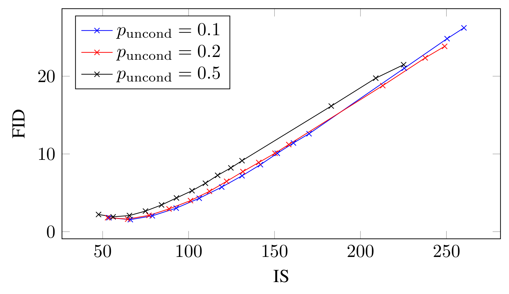
The horizontal axis is IS, not guidance weight; higher is better. The vertical axis is FID; lower is better. Legend values are training condition-drop probabilities p_uncond; points along each curve sweep inference guidance. Selecting only high IS can overlook worsening FID. This is a matched-evaluation trade-off plot, not an architecture diagram.
Jonathan Ho, Tim Salimans · 2207.12598v1 · Original paper · Figure in original · Enlarge Excerpt from the original paper. The figure region was cropped from the specified PDF version and rendered as a high-resolution PNG without redrawing its content. Commentary was written separately and translated for this edition. Rights remain with the original rights holders; the blog code’s MIT license does not grant redistribution rights to these figures.On the same page, Table 1 gives FID 1.80 at w_paper=0, 1.55 at 0.1, and 2.04 at 0.2 for p_uncond=0.1. Improvement followed by deterioration contradicts monotonic FID improvement with larger w. Read these through s=w_paper+1; they do not set 0.1 as optimal for every dataset. CFG v1, Figure 4 and Table 1, PDF p.7
#7.7 Beyond pixels: Latent diffusion
Latent diffusion first compresses spatial image information with an autoencoder, then learns denoising in that representation. Generation still needs repeated network evaluations: diffusion iterations run in latent space, and the final latent is decoded into an image separately. Rombach et al., 2112.10752v2, §3, Figure 3
Denoise in an autoencoder’s latent space rather than over all high-resolution pixels, then reconstruct with the decoder to reduce computation.
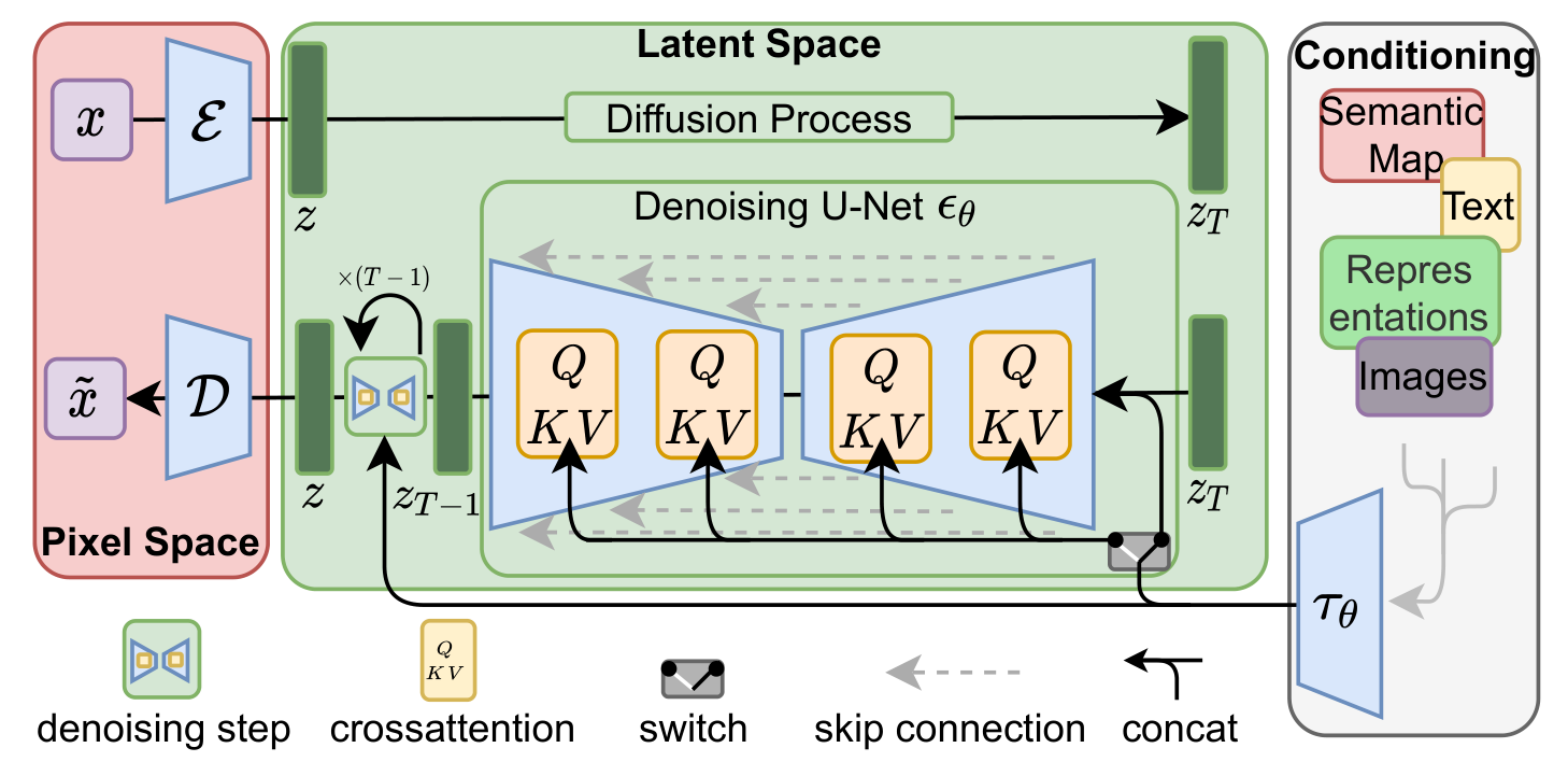
The red region E/D links images and latents; the green central region performs iterative diffusion and denoising. Conditions enter through concatenation or cross-attention depending on the task. In attention, image features supply Q and condition representations supply K/V. Distinguish the top diffusion arrows from the U-Net denoising path; not every condition enters identically.
Robin Rombach, Andreas Blattmann, Dominik Lorenz, Patrick Esser, Björn Ommer · 2112.10752v2 · Original paper · Figure in original · Enlarge Excerpt from the original paper. The figure region was cropped from the specified PDF version and rendered as a high-resolution PNG without redrawing its content. Commentary was written separately and translated for this edition. Rights remain with the original rights holders; the blog code’s MIT license does not grant redistribution rights to these figures.Connect Figure 3’s spatial regions to the compression example below. The diagram does not mandate 512×512 inputs and four latent channels for every LDM. Having encoder/decoder paths also does not mean both run at every inference denoising step. LDM v2, §3.2–3.3 and Figure 3, PDF p.4
Worked example — one f=8 configuration. Compress a 512×512×3 input to 64×64×4. Spatial positions decrease 262144→4096, to 1/64; scalars decrease 786432→16384, to 1/48. A “64-fold dimensional reduction” depends on whether channels are counted. Not all LDMs use f=8 or four channels; this is arithmetic for one chosen configuration.
Cross-attention conditioning can also be traced through tensors. The following explanatory notation describes one head, with L image positions, M text tokens, and head dimension d.
For L=4096, M=77, d=64, attention scores have shape 4096×77. Softmax normalizes over text tokens at each image position. Simply concatenating text onto image channels and producing 4096×4096 self-attention would be a different operation. The output supplies one feature per image position.
Read compression experiments in terms of reconstruction quality, generation quality, and training/sampling cost separately. The paper’s autoencoder and f-dependent generation comparisons examine losses in detail at excessive compression. Reconstruction FID differs from final generation FID. Scalar-count ratios do not establish speedups on untested hardware.
#7.8 A unified view through score matching and SDEs
A score is the log-density’s gradient with respect to input, not the training gradient with respect to model parameters. It is a local vector field toward higher density, not a probability or class confidence. Song et al., 2011.13456v2, §3–4
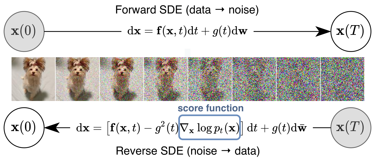
The upper arrow adds noise from x(0) to x(T); the lower generates from x(T) to x(0). The highlighted score enters the reverse drift and is estimated for time-varying distributions. The central image illustrates change, not guaranteed exact recovery of a particular photo. Figure 1 itself does not compare probability-flow ODE paths.
Yang Song, Jascha Sohl-Dickstein, Diederik P. Kingma, Abhishek Kumar, Stefano Ermon, Ben Poole · 2011.13456v2 · Original paper · Figure in original · Enlarge Excerpt from the original paper. The figure region was cropped from the specified PDF version and rendered as a high-resolution PNG without redrawing its content. Commentary was written separately and translated for this edition. Rights remain with the original rights holders; the blog code’s MIT license does not grant redistribution rights to these figures.Under Gaussian forward perturbation, the conditional score given x0 directly relates to injected noise as below. The noisy marginal score without x0 instead relates to the noise target’s conditional mean; do not substitute one sample value for both scores.
With barα=0.64, xt=−0.2, x0=0.5 as above, the conditional score is 5/3≈1.666667. If x0~N(0,1), the same VP perturbation preserves a marginal N(0,1), whose score at xt=−0.2 is 0.2. Different conditioning explains the different values.
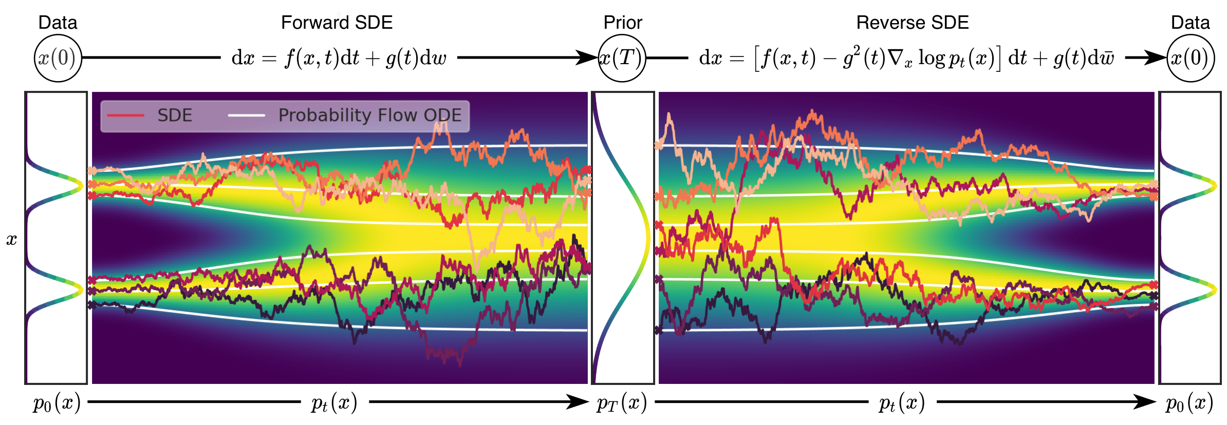
Both ends are data distributions; the center is the prior. Distinguish background distributions from individual sample paths. Rough SDE and smooth ODE paths need not coincide sample by sample. The connection concerns continuous-time marginal distributions; read it alongside the required 1/2 coefficient in the ODE’s score term below.
Yang Song, Jascha Sohl-Dickstein, Diederik P. Kingma, Abhishek Kumar, Stefano Ermon, Ben Poole · 2011.13456v2 · Original paper · Figure in original · Enlarge Excerpt from the original paper. The figure region was cropped from the specified PDF version and rendered as a high-resolution PNG without redrawing its content. Commentary was written separately and translated for this edition. Rights remain with the original rights holders; the blog code’s MIT license does not grant redistribution rights to these figures.With the paper’s scalar diffusion coefficient g(t), the reverse-time SDE is as follows. Here, integrating t from T to 0 makes dt negative. Switching to a positive reverse-time variable requires transforming drift signs.
The probability-flow ODE is not obtained merely by removing diffusion noise from the reverse SDE: its score coefficient is 1/2. Exact scores under continuous-time conditions can give matching timewise marginals, not identical individual paths. Learned-score and numerical-integration errors remain separate.
Worked example. For standard-normal score=−x and VP β=1, f=−x/2 and g²=1. Reverse-SDE drift is x/2; probability-flow ODE drift is 0. Since reverse dt<0, drift moves positive x toward the mean. Zero ODE drift is a special case where all timewise marginals already remain standard normal, not a claim that general image generation stays still.
Original Figure 1 illustrates forward/reverse SDEs, and Figure 2 relates SDEs to the probability-flow ODE. Section 4 describes numerical solvers such as predictor–corrector methods. Good sample quality reflects score model, architecture, and solver settings together. It is not evidence that changing SDE notation alone outperformed all earlier models. Both original conceptual figures are excerpted here, but do not establish solver rankings. Not every solver ablation was transcribed or training independently reproduced.
#7.9 Connecting the pieces
MMSE concerns optimal estimation under a specified loss; VAE learns an approximation to an intractable posterior; DDPM models reversal of a specified perturbation. CFG combines conditional and unconditional predictions, LDM changes the space in which iteration occurs, and Score-SDE explains noisy distributions and solvers in continuous time.
Keep prior versus posterior, α versus its cumulative product, analytic conditional posterior versus learned reverse distribution, original bound versus reweighted loss, code versus paper guidance scales, and spatial compression versus total tensor elements distinct. Implementation begins by substituting actual numbers to verify shapes, signs, and units, rather than memorizing one equation.