Contrastive representation learning designs what counts as the same entity and what serves as a comparison. Even identically named losses imply different training when positive definitions, candidate counts, gradient paths, or evaluation change. This article examines CPC, SimCLR, MoCo, and CLIP computations, connecting them to BYOL, Barlow Twins, clustering, and SupCon. Small matrices and numbers are separate explanatory examples, not paper results.
#8.1 From metric learning to contrastive learning
Distance-based learning constrains relationships among representations rather than only fitting class logits. A triplet compares relative distances among anchor a, positive p, and negative n.
Learn an embedding space with high similarity for semantically related views of an anchor and low similarity for other samples.
Worked example. With squared distances positive=0.2 and negative=0.3, and margin=0.5, the hinge loss is max(0,0.2−0.3+0.5)=0.4. If negative distance is 1.0, loss=0: sufficiently distant negatives give no gradient for this triplet. Selecting only harder negatives is not a universal answer. A different sample with the same real meaning may be a false negative, making its difficulty misleading supervision.
This triplet example differs from InfoNCE below. One penalizes margin violations; the other normalizes scores to identify a positive among candidates. Record each paper’s positive/negative sampling rules.
#8.2 InfoNCE: Classifying the correct pair
CPC encodes inputs and learns to distinguish related latents, such as future ones, from context. Original Figure 1 separates input encoding, autoregressive context aggregation, and future-representation scoring. Read CPC Figure 1 and §2, 1807.03748v2; do not present this overview as the same diagram as SimCLR with two augmented images.
For a candidate set containing one positive and negatives, write scores as s. The following expresses the loss in general softmax notation.
The positive appears in the denominator as well as the numerator. Calling the denominator a sum of negatives alone changes the probability and cross-entropy interpretation. For N equally scored candidates, positive probability is 1/N and loss log N; four candidates give approximately 1.386294 nats.
In the mutual-information lower bound, N is the total candidate count including the positive. Sampling assumptions, such as marginal negatives, also matter. Do not retain the original MI bound after arbitrary hard-negative mining. The bound’s log N limit does not guarantee that increasing N increases actual semantic information. CPC evaluates representation usefulness across domains, not generated-image FID. CPC, §2.3 and experiments
Implementation checks. Computing every exp first can overflow at large logits; use log-sum-exp. Distinguish temperature-scaled scores from raw cosine similarities. Check vanished effective negatives in tiny minibatches and false negatives from samples duplicated across distributed ranks.
#8.3 Augmentation defines the invariance to learn
Creating two views chooses which information may disappear while the views still count as the same. This is more than increasing dataset size. Consider downstream information removed by crops, color distortion, or blur. SimCLR, §3
Thought experiment. If an image contains a cat and a car but separate crops retain different objects, an instance-level positive is formed even though semantic equivalence is weaker. Strong color removal may likewise discard essential cues in color-sensitive defect detection. This is reasoning about data and objectives, not a reported experiment on that particular industrial dataset.
Specify augmentation ranges, positive-generation rules, available training information, and downstream goals together. Success on a standard benchmark does not justify uncritical reuse across all sensor, medical, or industrial images.
#8.4 SimCLR: A simple baseline sensitive to batch size and augmentation
SimCLR uses two augmented views of one image as positives and other batch views for comparison. Distinguish augmentation t, encoder f, and projection head g in the original framework. Chen et al., 2002.05709v3, §2, Figure 2
Treat two views of the same image as a positive pair and other views in the batch as negatives.
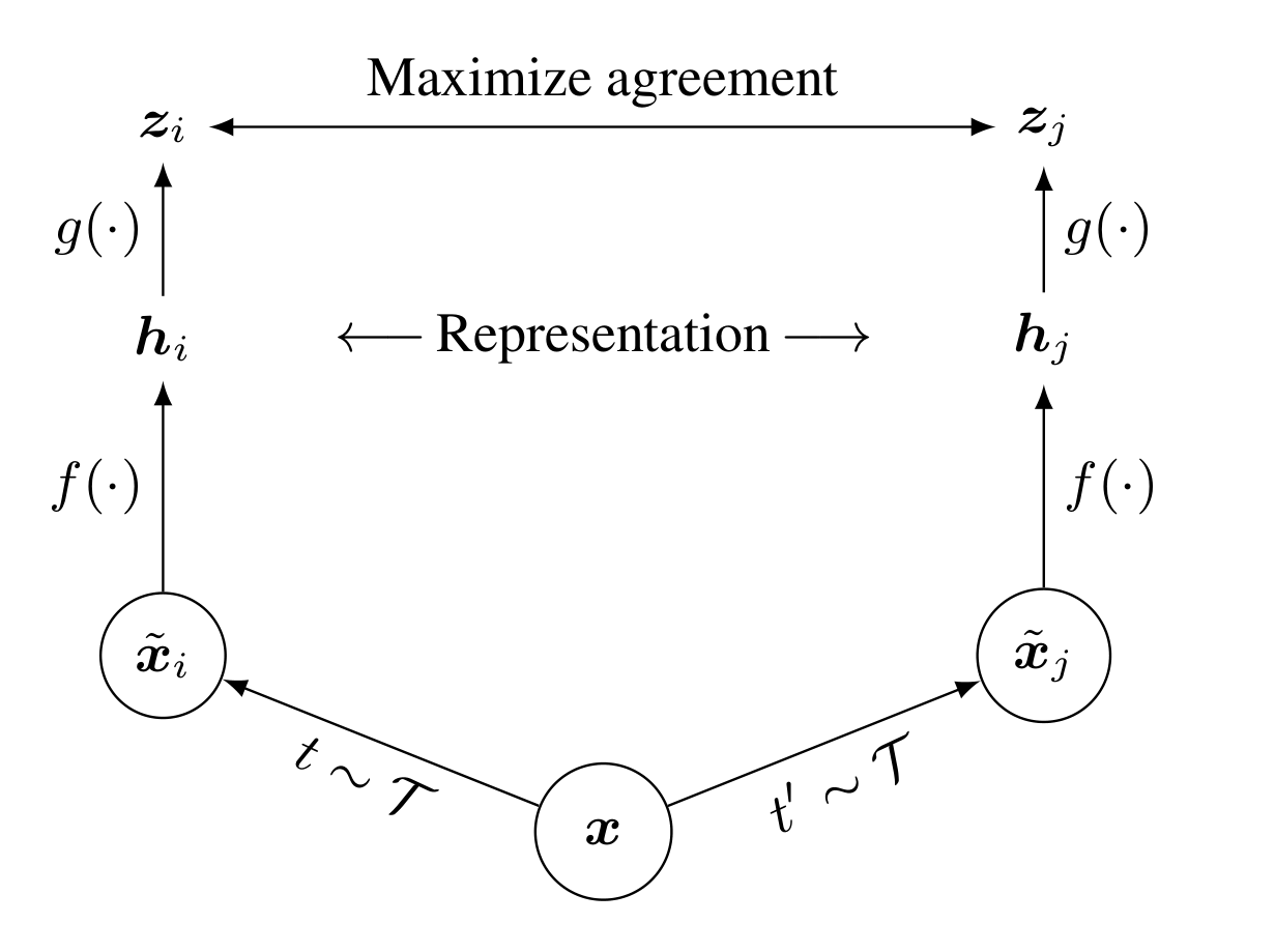
The two augmentations t and t′ are sampled independently. f and g have distinct roles, while both f branches share weights. Distinguish the objective trained at z from the choice to use h downstream.
Ting Chen et al. · 2002.05709v3 · Original paper · Figure in original · Enlarge Excerpt from the original paper. The figure region was cropped from the original PDF and rendered at high resolution. Commentary was written separately and translated for this edition. Rights remain with the original rights holders; the blog code’s MIT license does not grant figure redistribution rights.#N images, 2N views, and 2N−1 candidates
The preceding equation is cosine similarity. Substitution into the loss gives NT-Xent below; j(i) is anchor i’s positive index.
Two views per image yield 2N embeddings. Excluding only the anchor leaves 2N−1 candidates in the denominator: one positive and 2N−2 negatives. Symmetric training uses both directions, giving 2N anchors.
For N=2, order views as [a1,a2,b1,b2]. The positive for a1 is a2; negatives are b1 and b2. The denominator excludes a1 but includes a2. Reordering to [a1,b1,a2,b2] changes positive indices. Code assuming the target is always adjacent can fail under a different augmentation-concatenation order.
In an illustrative ResNet-50 shape example, pooled h is [2N,2048] and projection z is [2N,128]. Multiplying normalized z by zᵀ yields a [2N,2N] similarity matrix. The projection head creates a training comparison space; the paper’s linear evaluation uses h. SimCLR, §2, §4
#Checking temperature numerically
Suppose positive cosine similarity is 1 and the two negative similarities are 0 and −1. With τ=0.5, logits are [2,0,−2].
With τ=1, loss is approximately 0.407606. Here, lowering temperature concentrates probability on an already highest-scoring positive. A higher-scoring false negative would also be amplified. This calculation does not establish that smaller τ always yields better representations.
Let s_j be similarity before temperature division. The derivative is below; differentiating back to unnormalized embeddings also requires the normalization chain rule.
Memory example. For N=4096, an 8192×8192 matrix contains 67108864 elements; one float32 matrix occupies 256 MiB. This excludes gradients, encoder activations, and optimizer states, so it is not total GPU training memory. Blockwise computation can change implementation costs, but verify that the candidate set remains unchanged.
#Which model and evaluation produced the reported scores?
In Table 6’s ImageNet linear evaluation, standard ResNet-50 achieves 69.3% top-1 and ResNet-50(4×) 76.5%. These are not equal-sized backbones. Evaluation freezes the encoder and trains a linear classifier using labels, unlike CLIP zero-shot evaluation. SimCLR, Table 6, PDF p.7
Distinguish short ablations of projection, augmentation, and batch effects from final 1000-epoch results. Temperature/normalization comparisons also show that higher contrastive-matching accuracy need not mean higher downstream top-1. Record at least backbone width, epochs, batch size, h/z representation, and evaluation protocol.
#8.5 Can collapse be avoided without negatives?
If every input maps to the same vector, bringing positives together can leave no useful information. BYOL and Barlow Twins address this through different training structures. Sharing the absence of explicit negatives does not imply the same mathematical objective.
BYOL uses stop-gradient and a momentum target; Barlow Twins aligns the diagonal and suppresses off-diagonal terms of cross-correlation.
#Barlow Twins: D×D features, not N×N samples
Barlow Twins pushes cross-correlation between two view representations toward identity. In original Figure 1, encoder paths meet at a feature-correlation matrix, not class scores or an instance-similarity table. Barlow Twins, 2103.03230v3, Figure 1 and §2
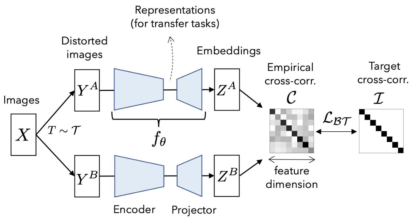
The right matrices are empirical cross-correlation C and target identity I. Axes are feature dimensions, not image IDs. Diagonal terms align matching dimensions across views; off-diagonal terms address redundancy. Unlike BYOL’s online/EMA target, these paths apply the same network to two views. Distinguish downstream representations from projections as well.
Jure Zbontar, Li Jing, Ishan Misra, Yann LeCun, Stéphane Deny · 2103.03230v3 · Original paper · Figure in original · Enlarge Excerpt from the original paper. The figure region was cropped from the specified PDF version and rendered as a high-resolution PNG without redrawing its content. Commentary was written separately and translated for this edition. Rights remain with the original rights holders; the blog code’s MIT license does not grant redistribution rights to these figures.For batch size B and projection dimension D, both representations are B×D and correlation is D×D. Center each feature and normalize using its squared sum over the batch to compute C_ij. Diagonal terms align the same feature across views; off-diagonal terms reduce feature redundancy.
Worked example. With C=[[1,0.2],[0.2,1]] and λ=0.005, diagonal cost=0 and off-diagonal cost=0.005×(0.04+0.04)=0.0004. A value of 0.0002 omits half the terms when both i,j and j,i are summed. If C is all zero, diagonal cost is D. Constant features have zero variance and undefined normalization, so explain the implementation’s ε handling.
Evaluations and ablations examine invariance, redundancy, and projection effects. The loss form alone does not prove collapse impossible for every batch and optimizer. Test small-batch correlation estimates and zero-variance handling separately.
#BYOL: The optimizer does not jointly move the target
In original Figure 2, the online path is encoder → projector → predictor; the target path is encoder → projector. Target representations receive stop-gradient, and target parameters follow an EMA of online parameters. Add the loss with augmented-view roles swapped. BYOL, 2006.07733v3, Figure 2 and §3
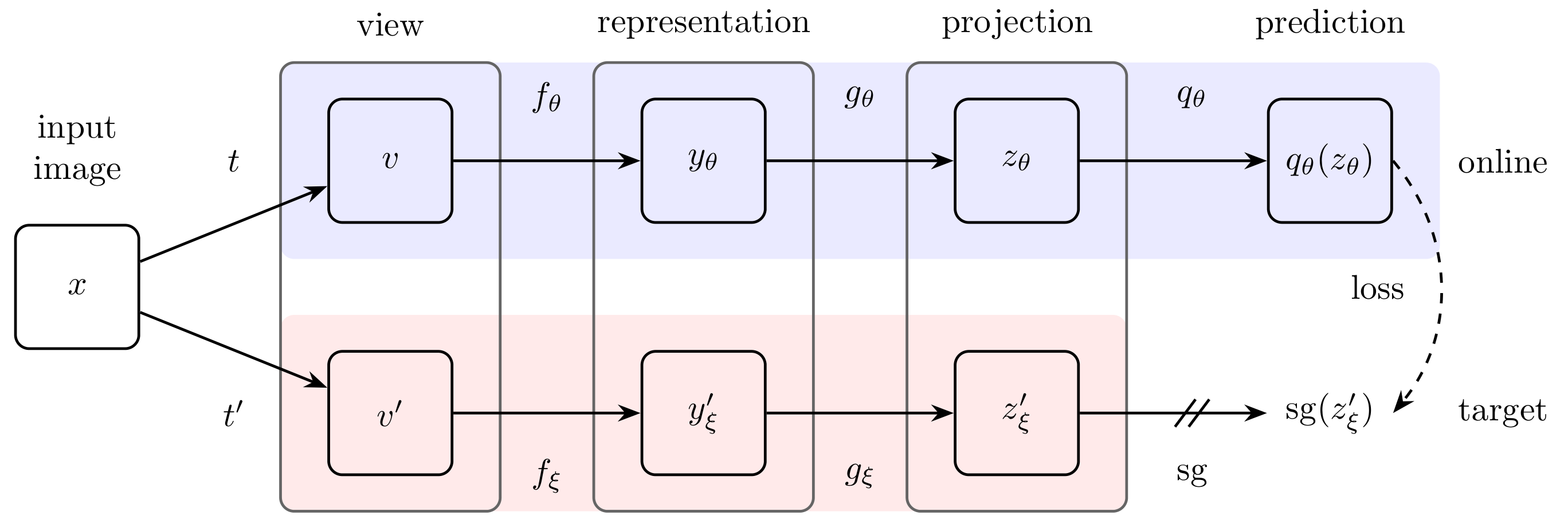
The upper prediction is qθ(zθ); the lower target is sg(z′ξ). Stop-gradient blocks backpropagation in that direction, not target updates forever. The EMA rule is given separately below. The figure shows one direction; swap view roles for the symmetric loss. The retained representation after training is the online encoder’s yθ.
Jean-Bastien Grill et al. · 2006.07733v3 · Original paper · Figure in original · Enlarge Excerpt from the original paper. The figure region was cropped from the specified PDF version and rendered as a high-resolution PNG without redrawing its content. Commentary was written separately and translated for this edition. Rights remain with the original rights holders; the blog code’s MIT license does not grant redistribution rights to these figures.For normalized prediction u and target v, squared distance relates to cosine as follows. Equality assumes both are unit vectors.
Worked example. Cosine=0.8 gives one-way loss 0.4. Reverse cosine=0.6 gives 0.8, for sum 1.2 or mean 0.6. Distinguish two directions from loss reduction. With old target 0, online value 2, and m=0.9, new target is 0.2. This is a scalar illustration, not a claim that the paper has one parameter.
Including target parameters in the optimizer changes the original stop-gradient structure; fixing them forever also differs from EMA. The paper observes useful learning in its proposed setup despite possible collapsed objectives, and examines bootstrapping/predictor ablations. Do not generalize this into a proof that EMA alone prevents collapse for any model. Its ResNet-50 linear-evaluation score of 74.3% cannot isolate a module’s effect by subtraction from differently trained/evaluated papers.
Both original diagrams are excerpted and connected to losses and gradient paths. The diagrams themselves neither prove collapse prevention under every setting nor constitute ablation tables. Not all ablation numbers were transcribed or independent training performed.
#8.6 Memory banks and MoCo
Using only current-batch views ties candidate count to batch size. Stored keys enlarge the set, but rapid encoder changes can put old keys and current queries in mismatched representations. MoCo addresses a large dictionary together with consistency over time. He et al., 1911.05722v3, §3
Update the query encoder by gradients and the key encoder by moving average. Retain previous batches’ keys in a queue to use many negatives consistently.
#Reading original Figure 1 through the queue’s lifetime
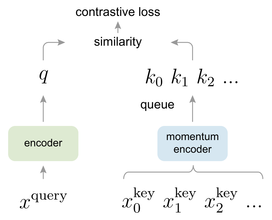
Compare q at left with the encoded-key dictionary at right. The queue stores embeddings; the text defines insertion of new minibatches and removal of old ones. Gradient learning for queries differs from momentum updating for the key encoder. This overview does not enumerate every queue state over time.
Kaiming He, Haoqi Fan, Yuxin Wu, Saining Xie, Ross Girshick · 1911.05722v3 · Original paper · Figure in original · Enlarge Excerpt from the original paper. The figure region was cropped from the specified PDF version and rendered as a high-resolution PNG without redrawing its content. Commentary was written separately and translated for this edition. Rights remain with the original rights holders; the blog code’s MIT license does not grant redistribution rights to these figures.In original MoCo Figures 1 and 2, distinguish queries, current-batch positive keys, and historical queue keys. Incoming keys are enqueued; old keys are dequeued. The queue stores computed key embeddings, not original images. Reading it as an image replay buffer miscalculates memory and gradients. Read Figure 1’s overview together with Figure 2’s gradient comparison.
The query encoder learns by gradients; the key encoder updates slowly through EMA. Historical embeddings are not recomputed with the latest encoder each time. Rather than claiming all keys come from an identical encoder, say gradual changes reduce inconsistencies among keys.
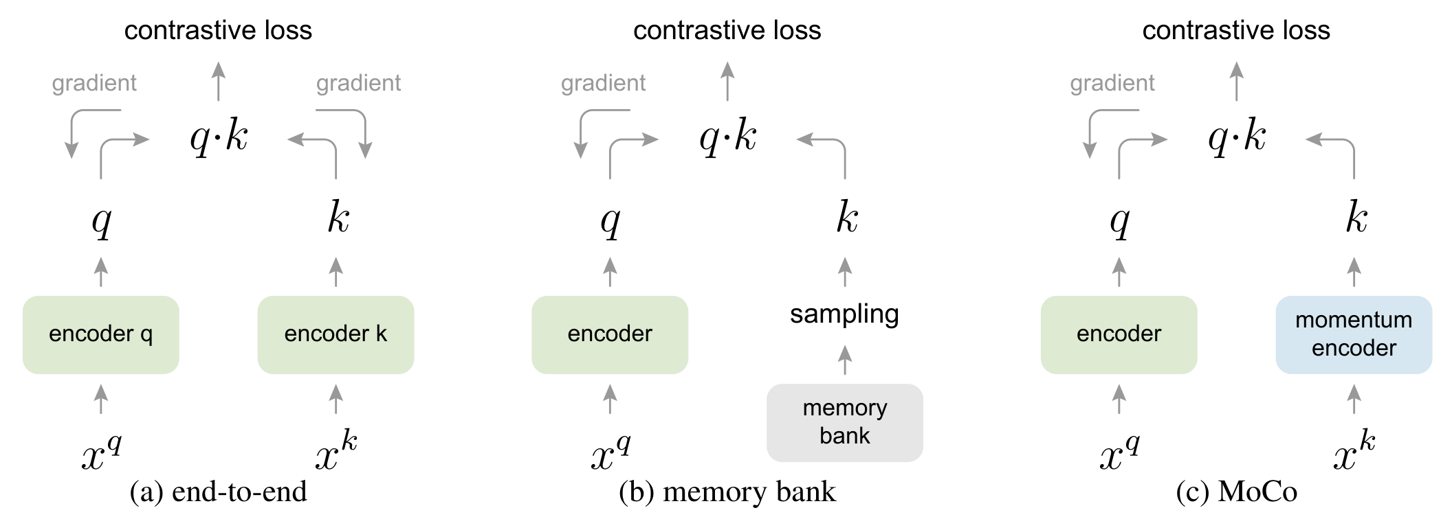
In (a), backpropagation updates both encoders; (b) retrieves stored keys from a memory bank; (c) creates new keys with a momentum encoder. The caption explicitly says the queue is not drawn in Figure 2. Do not invent absent queue arrows; connect the figure to Figure 1 and the text. It compares concepts, not numerical performance gaps.
Kaiming He, Haoqi Fan, Yuxin Wu, Saining Xie, Ross Girshick · 1911.05722v3 · Original paper · Figure in original · Enlarge Excerpt from the original paper. The figure region was cropped from the specified PDF version and rendered as a high-resolution PNG without redrawing its content. Commentary was written separately and translated for this edition. Rights remain with the original rights holders; the blog code’s MIT license does not grant redistribution rights to these figures.For illustrative query Q of B×d, positive K+ of B×d, and queue K×d, positive scores are B×1 and negative scores B×K. Combined logits are B×(1+K). Putting positives first makes all targets index 0, an implementation convention determined by storage order.
#Queue length differs from EMA memory length
Worked example. With K=65536 and 256 global keys inserted per step, the queue turns over in 256 steps. For EMA m=0.999, the steps until old-parameter influence halves are given below.
256 and approximately 693 describe different memories: replacement of stored embeddings versus persistence of old parameter states in EMA. Converting either to epochs also requires dataset size and global batch size.
At m=1 the key encoder never updates; at m=0 it immediately follows the query encoder. Which extreme works depends on training. The paper examines dictionary-size and momentum ablations. Do not mix projection/augmentation changes from other versions into “original MoCo.”
#When implementation order changes the loss
Following the original operations, compute current queries and positives, select a snapshot of the historical queue for this loss, then calculate scores. Enqueuing new keys first can place the same positive among negatives and change the denominator. Specify query gradients, no-grad key computation, EMA/enqueue timing, and global key count after distributed all-gather.
MoCo’s shuffling BN reduces shortcuts through batch statistics. It does not randomly change correct pairs; key sample ordering must be restored. Stored queue tensors are not optimizer-updated parameters.
Reading the experiments. MoCo evaluates transfer to detection and segmentation as well as frozen-feature linear classification. Good linear top-1 differs from good detector fine-tuning. Compare supervised pretraining under matched detector architecture, fine-tuning schedule, and initial normalization. This expansion explains principles and ablation questions; it does not retranscribe every detector table or reproduce experiments. MoCo, §4.1–4.2
#8.7 Feature clustering: DeepCluster and SwAV
#DeepCluster: Learning the next representation from labels produced by the current one
DeepCluster alternates clustering current features and using resulting assignments as pseudo-labels to train the encoder. Read its overview as repeated feature extraction → clustering → pseudo-label training. DeepCluster, 1807.05520v2, §3
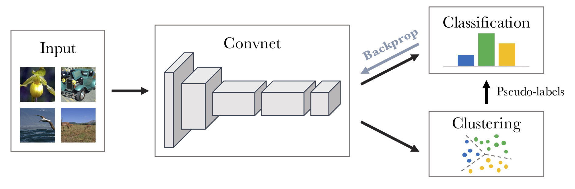
Clustering at lower right supplies classification pseudo-labels above, whose backpropagation updates the ConvNet. Separate assignment generation from learning with fixed pseudo-labels. The diagram does not make discrete cluster selection one differentiable layer, nor fix cluster IDs to semantic class names.
Mathilde Caron, Piotr Bojanowski, Armand Joulin, Matthijs Douze · 1807.05520v2 · Original paper · Figure in original · Enlarge Excerpt from the original paper. The figure region was cropped from the specified PDF version and rendered as a high-resolution PNG without redrawing its content. Commentary was written separately and translated for this edition. Rights remain with the original rights holders; the blog code’s MIT license does not grant redistribution rights to these figures.A simplified k-means stage follows. With the encoder fixed, find centroids and assignments; in the next stage, use assignments as training targets. Keep these optimization problems distinct.
Worked example. Splitting one-dimensional features [0,0.2,3,3.2] into two clusters gives centroids 0.1 and 3.1. Swapping cluster IDs 0 and 1 leaves the partition unchanged. If IDs change at the next clustering step, do not assume the previous classifier’s classes retain their meanings. Define rules for dominant and empty clusters too.
Experiments evaluate downstream transfer and design choices, not a guaranteed one-to-one match between pseudo-labels and semantic classes. This discussion explains the algorithm and collapse risks without reconstructing every downstream numerical table.
#SwAV: Predicting one view’s assignments from another view’s prototypes
SwAV swaps prototype assignments across views for prediction, rather than directly comparing negatives across all instance pairs. Follow the crossed supervision between predictions and assignments in original Figure 1. SwAV, 2006.09882v5, §3
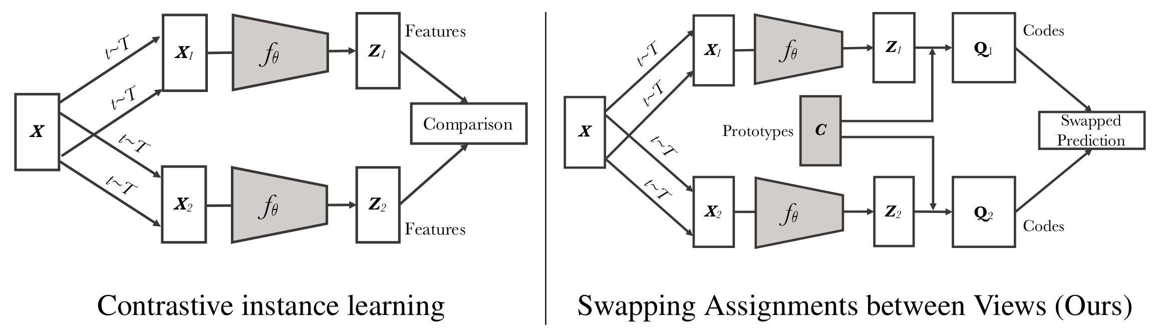
C at right denotes prototypes; q1/q2 are codes for each view. Cross-supervision supplies one view’s code to the other’s prediction. This cannot be reduced to directly increasing two-feature similarity as at left. Distinguish assignment constraints from prediction cross-entropy to understand the Q mass normalization below.
Mathilde Caron, Ishan Misra, Julien Mairal, Priya Goyal, Piotr Bojanowski, Armand Joulin · 2006.09882v5 · Original paper · Figure in original · Enlarge Excerpt from the original paper. The figure region was cropped from the specified PDF version and rendered as a high-resolution PNG without redrawing its content. Commentary was written separately and translated for this edition. Rights remain with the original rights holders; the blog code’s MIT license does not grant redistribution rights to these figures.For N embeddings of dimension D and K prototypes, predictions form N×K. Let Q∈R^(K×N) be the normalized mass matrix for balanced assignment, with marginal constraints below. To obtain per-sample probabilities, distinguish the convention of multiplying each column by N so its sum becomes 1.
Worked example. With K=N=2 and diagonal Q entries 0.5, all others zero, total mass is 1 and both constraints hold. Each Q column sums to 0.5, not 1. In contrast, 2Q gives one-hot assignments per sample. Confusing the two mis-scales cross-entropy with batch size.
With assignments qA/qB and predictions pA/pB for views A/B, one swapped-loss pair is below, restating the paper’s notation.
Balance constraints regulate prototype use; they do not establish uniform real-world class frequencies. The paper studies online clustering, multi-crop, and related settings. Do not attribute every improvement solely to the absence of negatives. This expansion covers the core objective and mass conservation; Sinkhorn numerical stability and full ablations remain further topics.
#8.8 With some labels: Supervised contrastive learning
SupCon uses samples sharing the anchor’s class as positives. It does not assume true shared classes can automatically be known without labels. SupCon, 2004.11362v5, §3
The paper’s principal form averages log probabilities over positives, which differs from taking log after averaging positive probabilities. The denominator excludes only the anchor; other positives remain.
Worked example. Suppose two positives have softmax probabilities 0.2 and 0.6. Mean negative log is 1.060132; negative log of mean probability is 0.916291. The objectives penalize unevenly matched positives differently.
Specify how anchors with no valid positive are handled in partially labeled batches. Avoid division by empty-set sizes, and align positive masks with distributed sample ordering. The results support supervised representation learning, not universal removal of all within-class diversity. This expansion compares objectives without retranscribing every backbone’s best scores.
#8.9 CLIP: Extending positives to image–text pairs
CLIP learns image–text pairs rather than only two augmented views of an image. After training, label descriptions pass through the text encoder for comparison with images. This differs from an autoregressive decoder generating image captions. The consulted Radford et al. version is 2103.00020v1. CLIP, §2, Figure 1
Construct an N×N similarity matrix between N images and N texts in a batch, then train with bidirectional cross-entropy to emphasize the correct diagonal pairs.
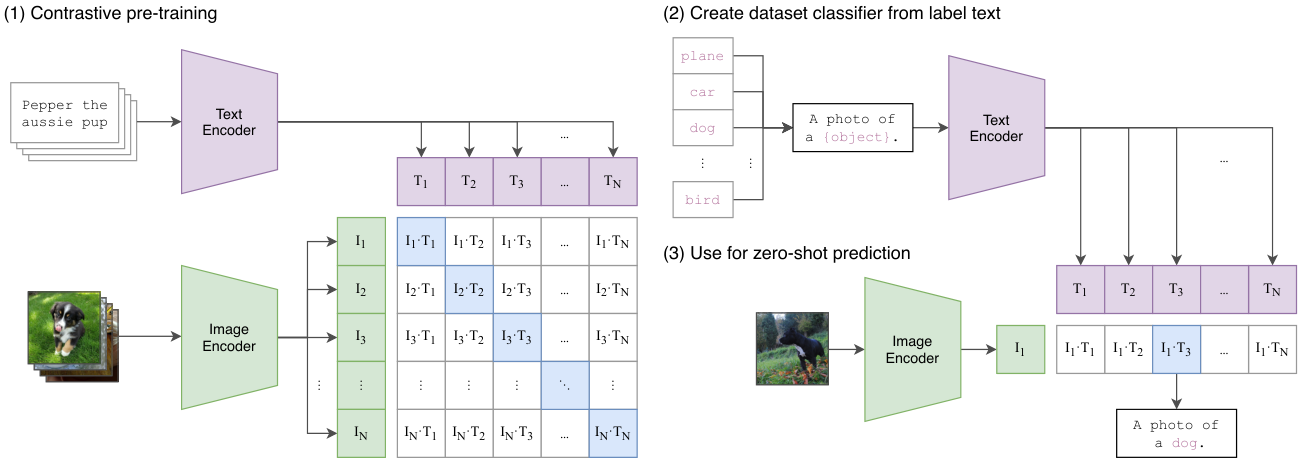
The large left table is the training image–text similarity matrix; diagonal pairs provide supervision. Upper right, label texts create classifier comparison vectors; lower right, a new image is compared with them. Distinguish training captions from inference class prompts.
Alec Radford et al. · 2103.00020v1 · Original paper · Figure in original · Enlarge Excerpt from the original paper. The original PNG is used unchanged. Commentary was written separately and translated for this edition. Rights remain with the original rights holders; the blog code’s MIT license does not grant figure redistribution rights.#Two encoders and bidirectional cross-entropy
If projected, normalized image embeddings I and text embeddings T are each N×D, logits are N×N. With learned log scale t, write them as below. t itself is not temperature; exp(t) is the inverse-temperature logit scale.
Rows seek each image’s correct text; columns seek each text’s correct image. This convention averages both directions. Do not remove the diagonal as self-similarity as in SimCLR: CLIP’s diagonal contains correct image–text pairs. Each row has one positive among N candidates, hence N−1 negatives.
Worked example. With two-pair logits [[2,0],[0,2]], loss in each direction is log(1+exp(−2))≈0.126928, as is their mean. Masking the diagonal deletes targets. Logit 2 is illustrative, not a claim about a pretrained CLIP temperature.
#Tracing zero-shot classifier shapes
For B inference images and K candidate classes, image features are B×D and label-prompt features K×D; their product is B×K. Training batch size N need not equal test class count K. Explain sentence templates and where normalization occurs when averaging prompts.
A high dog score among dog/cat differs from a high dog probability among dog/cat/wolf/fox/bear. Softmax probabilities depend on the candidate set. Similarity to the best-matching sentence differs from an absolutely calibrated recognition confidence.
What the paper examined—and what it did not. CLIP compares large-scale image–text pretraining through zero-shot and linear-probe evaluation across downstream datasets. Zero-shot means no classifier fitting with target-task training labels; it does not mean no pretraining data, language supervision, or bias. The paper also examines prompt engineering and dataset shift. CLIP, §3
Differences between SimCLR linear-probe top-1 and CLIP zero-shot top-1 cannot be attributed solely to representation quality. Supervised heads, pretraining data, backbones, resolution, and prompts also vary. Repeatedly tuning prompts against a test set compromises evaluation independence despite the zero-shot label. This is an evaluation-design consideration, not a claim of guaranteed deployment calibration.
#8.10 Choosing a method
| Situation | Method to examine first | Key verification question |
|---|---|---|
| Contrast two views in one batch | SimCLR | Are positives included in the denominator, self-masking correct, and h/z distinguished? |
| Small batches with a large dictionary | MoCo | Are queue lifetime, EMA timing, and key gradients correct? |
| Avoid explicit negatives | BYOL/Barlow Twins | Are target updates, stop-gradient, and correlation axes correct? |
| Iterative prototype learning | DeepCluster/SwAV | Are assignment meaning, balance, and mass normalization correct? |
| Use labels to define positives | SupCon | Are positive log probabilities averaged, and empty positive sets handled? |
| Image–text zero-shot comparison | CLIP | Is the diagonal retained as targets, and evaluation distinguished from task-label fitting? |
This is a reading and implementation checklist, not a new benchmark ranking. Recording each paper’s positive/negative definitions, stored tensors, gradient paths, summed/averaged losses, and pretraining/downstream data use reveals the actual differences behind the shared name “contrastive learning.”