This lesson picks up the model that distinguishes objects pixel by pixel in Robot Learning 01. A robot reaching for a cup needs two pieces of information: whether a cup is present and which pixels belong to it.
We will read the semantic segmentation section of Stanford CS231n 2026 Lecture 9, one slide at a time, from PDF pages 32 through 64. Under each original slide, the commentary explains the figure, the operation it illustrates, and what changed from the preceding slide. This section is part of a 147-page lecture. The slides retain their author and image credits. Worked examples created for this article are identified separately.
Official course schedule · Original PDF · Supplementary video: Stanford Online 2025 Lecture 9
The video is from 2025 and the slides are from 2026. The topic links below use the manually prepared English captions from the 2025 recording. Their timestamps mark spoken explanations. They do not specify when the slides in the 2026 PDF change. The accompanying prose is original commentary. For more on the architectures, papers, and equations, see Modern AI VI.
Segmentation and reinforcement learning answer different questions. Segmentation is a perception task. Reinforcement learning uses actions, outcomes, and rewards to learn how to make decisions. A policy can use segmentation as part of its observation, and some policies learn directly from other inputs.
#P032. Four ways to describe the same scene
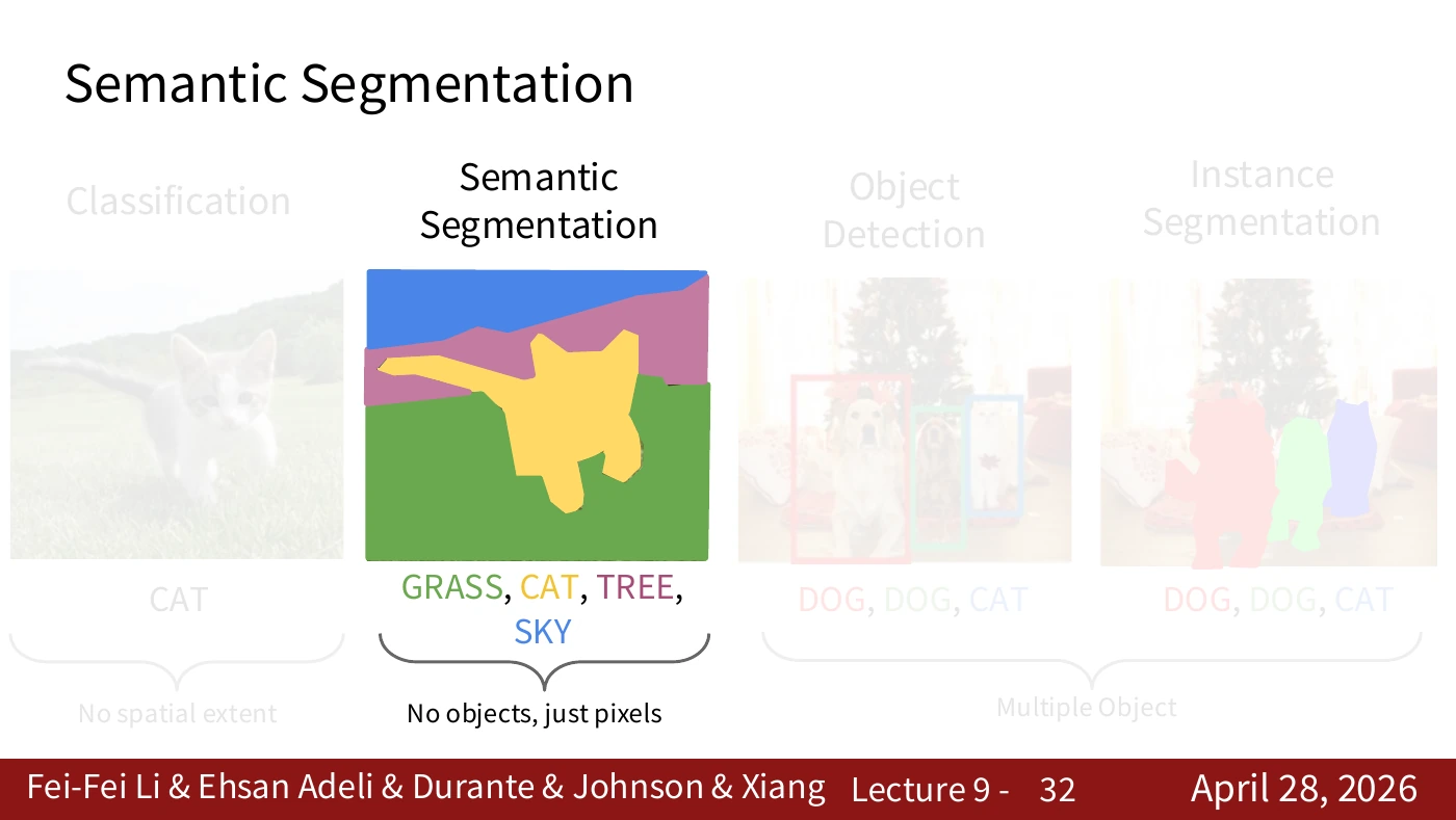
A classifier assigns a label to an image. A detector returns a box for each object. Semantic segmentation assigns a category to each pixel. Instance segmentation produces a separate mask for each object. Imagine a robot choosing between two cups. Labeling every cup pixel answers one question. Separating those pixels into two distinct cups answers another.
The slide highlights semantic segmentation and fades the other three tasks to mark the topic of this part of the lecture. Before moving on, explain why two separate objects in the same category can have the same color in a semantic mask.
#P033. A ground-truth category for each pixel
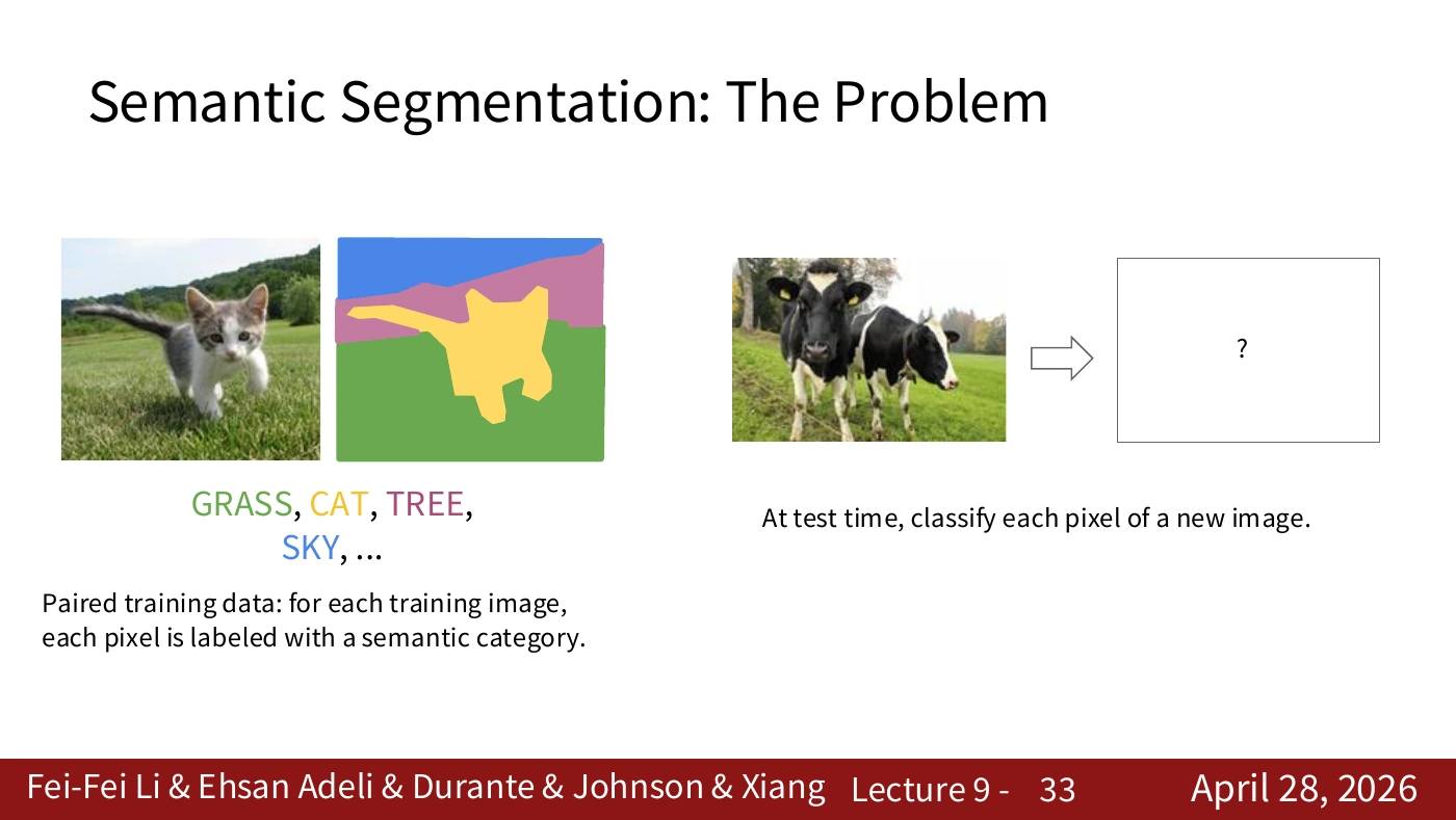
Each training image is spatially aligned with its label map. Given a new image, the model predicts a category at each pixel. It can use the surrounding context to make that prediction. The dataset’s annotation rules for occlusions and boundaries also affect what counts as the correct label.
On the left are image–label pairs used in training. The question mark on the right is the map the model must predict from a new image, without the training labels as an input. When cropping or resizing an image and its ground truth, apply the same coordinate transformation to both.
#P034. Which pixel are we classifying?
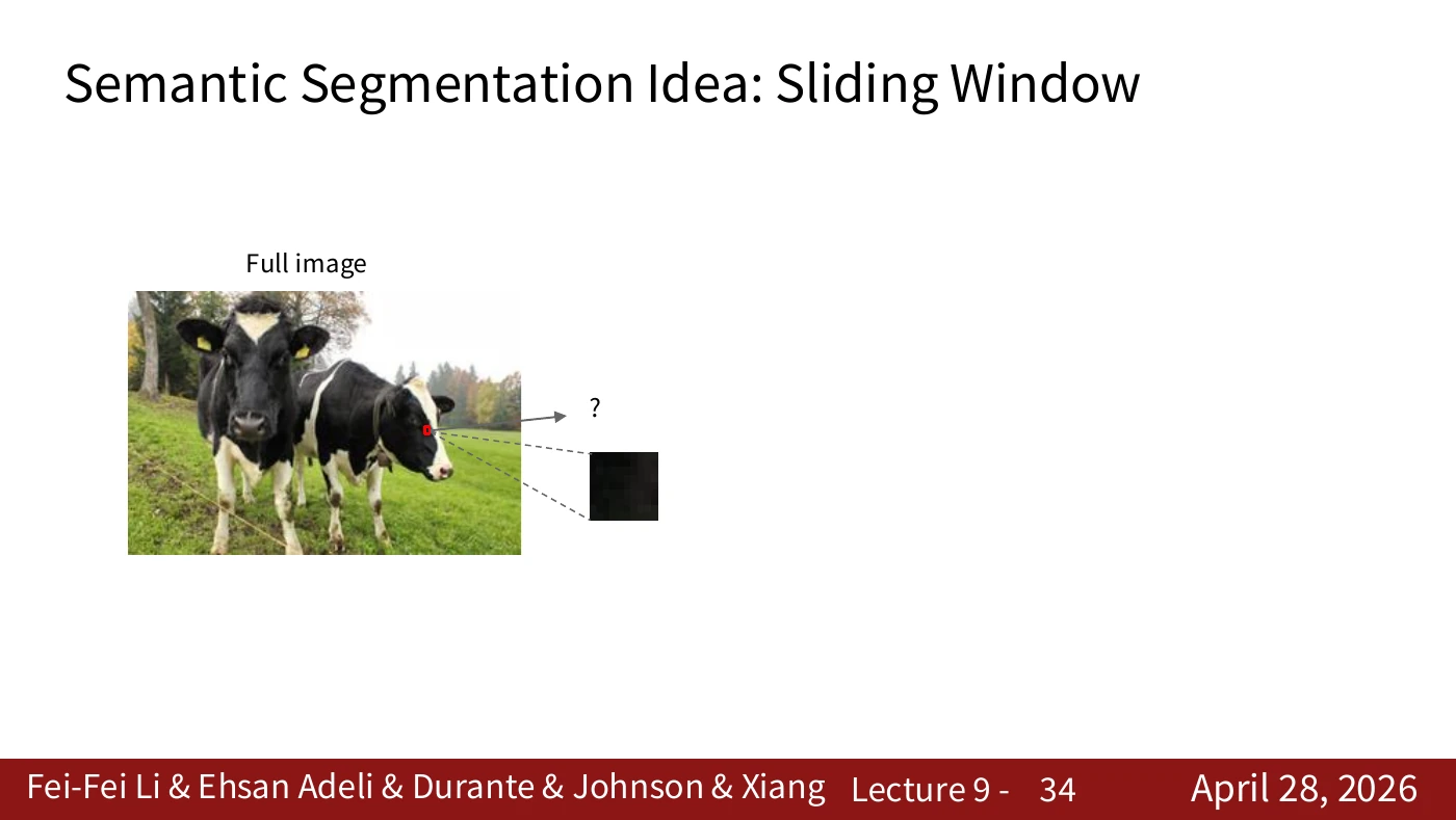
Find the location marked with a question mark. The task now asks for the category at that position. The slide establishes what to predict before considering how to design an efficient network.
The enlarged black square gives little evidence about whether it belongs to an object or a shadow. Locate it in the original image, then cover the surroundings. Can you still identify it? This small exercise exposes the context problem in the next slide.
#P035. Why the surrounding pixels matter
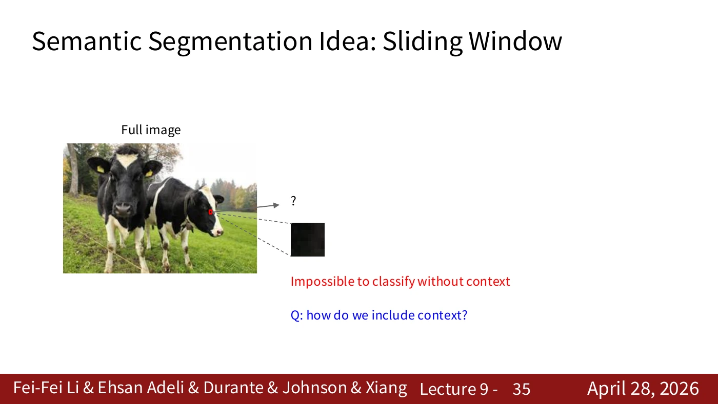
A single color gives weak evidence for a category such as cow or grass. Many objects share the same colors. A larger window brings in more context, at the cost of additional computation and choices about how to handle image edges.
The red text identifies the difficulty of classifying a pixel in isolation. The blue question asks how to supply context. First identify the missing information. The choice of model comes next.
#P036. Giving context to the model
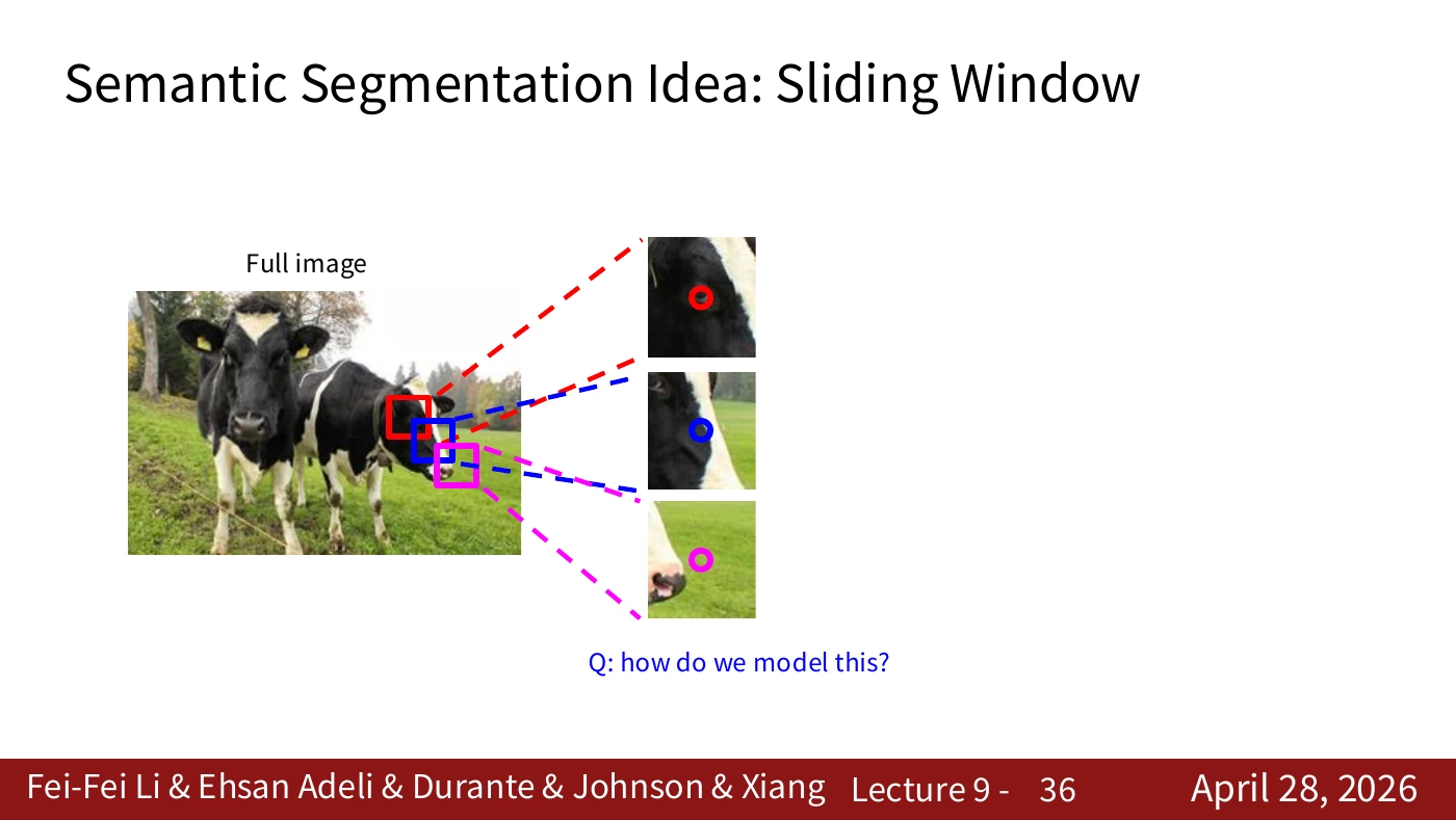
To use nearby pixels, we need to turn a neighborhood into a model input. Even when a prediction concerns just the center pixel, the input can contain a whole patch. This is the link to patch classification on the next slide.
The red, blue, and pink windows mark different positions in the same image. Distinguish the input window from the label of its center pixel. A model can learn to label this designated position even when a different category dominates the patch.
#P037. Classifying the center pixel with a patch and a CNN
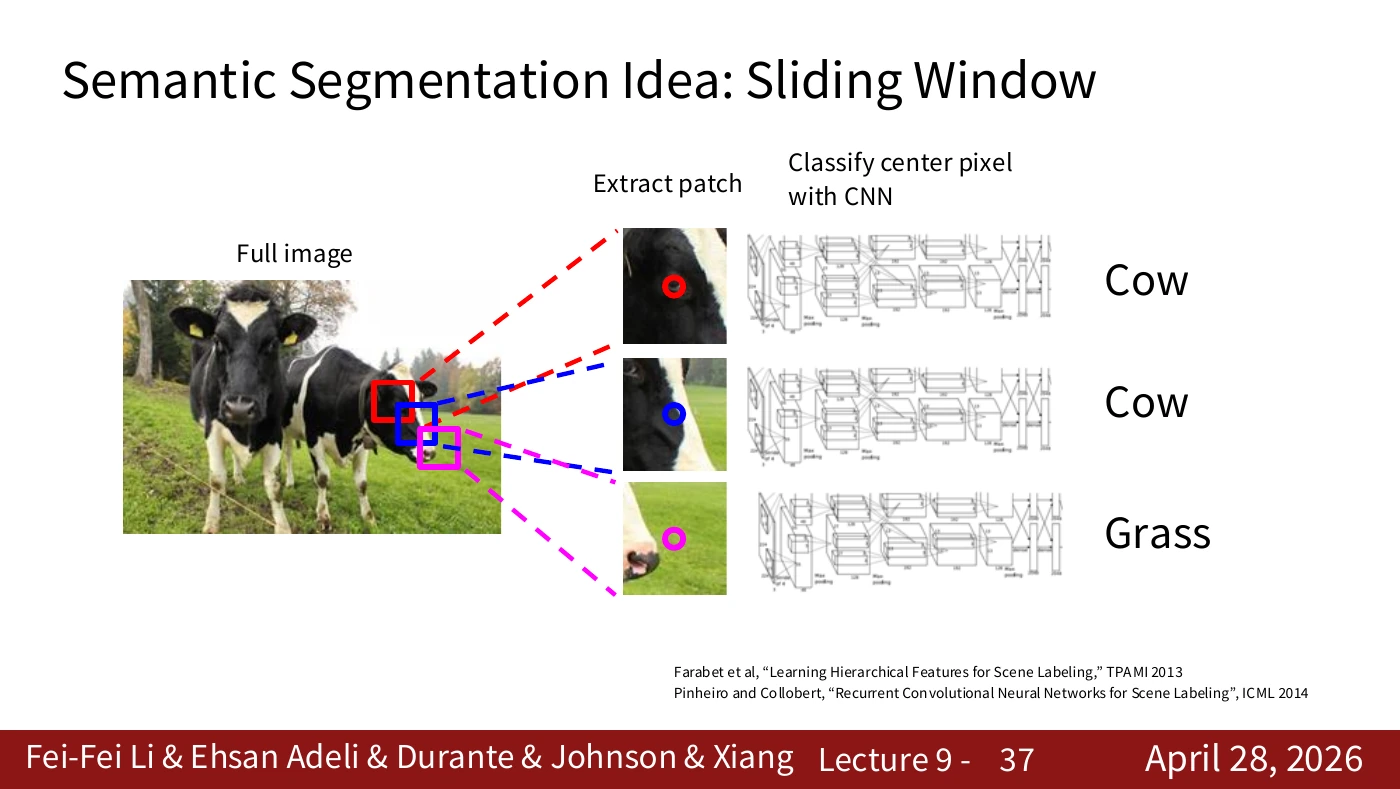
Crop a small window, pass it through the CNN, and read the category at its center. This yields one prediction. Repeating the operation over many center positions produces a spatial label map.
The two upper windows correspond to the cow and the lower window to grass. All positions use the same CNN and share its weights, including positions whose centers belong to different classes.
#P038. Overlapping windows repeat work
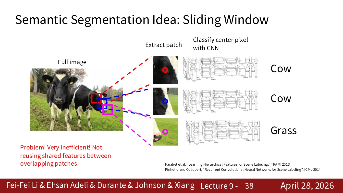
Neighboring windows share much of their input. Running a CNN independently on each window repeatedly extracts similar low-level features. The computational cost comes from the missed opportunity to share work. Later slides reuse features computed over the whole image.
Shift a 31×31 window one pixel to the right and 30 columns still overlap. Starting every convolution from scratch would recompute features in that shared area. The speedup depends on the architecture and implementation. The overlap shows where savings are possible.
#Video supplement · Using context and sharing computation
The 2025 lecture, 18:26–20:27, treats two problems in sequence. First, one green pixel could be grass or green clothing. The surrounding shape and texture provide evidence. This motivates the larger windows and patch classifier on P034–P037. Second, moving the window one position makes the model read most of the same pixels again. Obtaining context still leaves repeated computation to address.
A network run independently at every location of a 100×100 image has 10,000 target positions. Neighboring targets can have different labels even when their patches overlap. Much of the early edge and texture computation can nevertheless be shared. The transition to a fully convolutional network (FCN) preserves context by reusing features computed over the entire image.
#P039. Connecting a classifier’s coarse grid to pixel locations
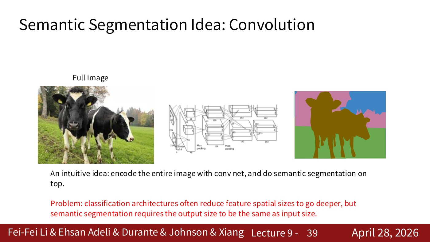
Classification networks often reduce feature-map resolution with depth. Segmentation requires an output at each target position, so coarse features must be mapped back to image coordinates. The design needs a spatially indexed output even when it encodes the whole image in one pass.
Follow the arrow from the whole-image encoding to the spatial prediction map. If the network reduces output resolution, the predictions need upsampling and alignment. Taking the final image-level classification alone does not produce a label map.
#P040. Computing C scores at each location
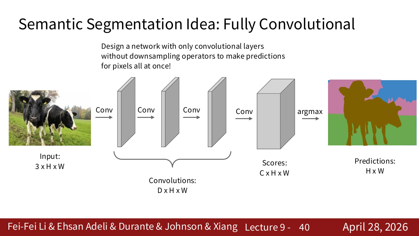
A 3×H×W input yields a C×H×W score map. Taking the argmax over the class channels gives an H×W prediction. C is the number of categories. The argmax returns a class ID. During training, the loss compares logits with ground truth, rather than measuring distances between discrete IDs.
D on the slide is the number of intermediate feature channels. C is the number of output categories. They can differ. The final argmax retains the spatial grid, selecting one of C classes at each location. The worked example below returns to the difference between a probability and a class ID.
#Supplementary lecture and paper · Turning a classifier into an FCN
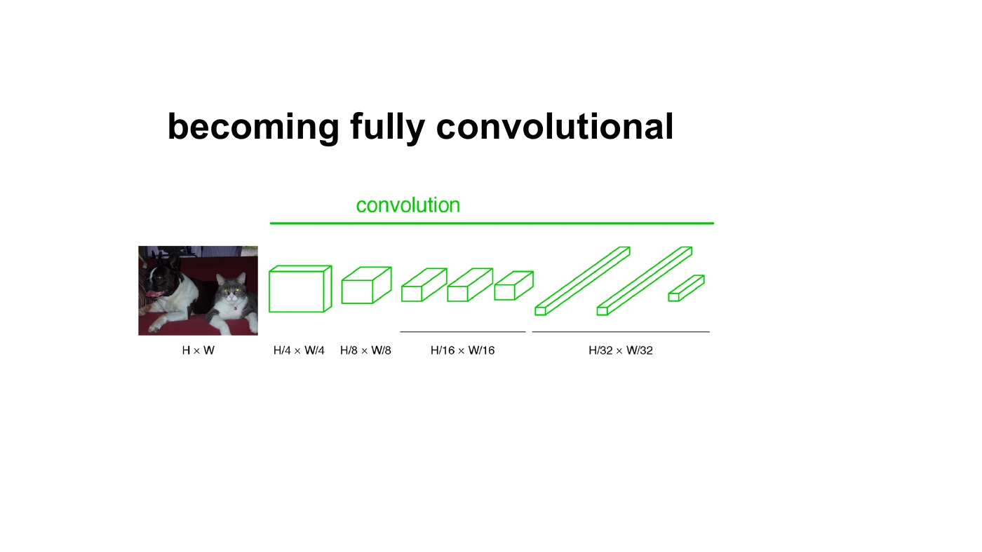
The figure makes the spatial dimensions behind P040 explicit. H and W shrink, but several output locations remain on the right. For example, take a 320×320 input and a network with an overall stride of 32. Under a simplified boundary rule, the output grid is 10×10. With K class scores per location, its shape is K×10×10. Upsample and align that grid to the input resolution to use the scores for pixel-level prediction.
Sections 3 and 4 of the FCN paper show how to retain the learned features of a classifier and apply them on a spatial grid for dense prediction. Even fully connected weights can operate as convolutions when interpreted with the corresponding kernel shape. The term fully convolutional allows different feature-map sizes throughout the network. Pooling and strided layers can produce a coarse grid.
Can we simply enlarge the coarse result? The names FCN-32s → FCN-16s → FCN-8s describe architectures that fuse predictions from progressively finer intermediate grids to improve localization. The numbers do not count layers. Deeper layers help identify an object, while shallower layers can retain evidence about its boundaries. The 2015 experiments illustrate this principle within their own evaluation settings.
The 2025 video, 20:57–22:13, explains the name FCN and its downsampling and upsampling paths. On P041–P043, track where the spatial score map becomes coarse and where it becomes dense again.
#P041. The cost of computing at full resolution
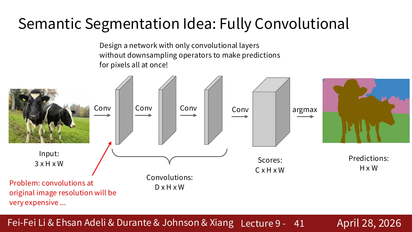
Keeping locations available throughout a network carries a cost. Many convolutions on a large H×W grid can be expensive. Read the advantage of dense spatial information alongside the cost set by channels, kernels, and resolution.
Doubling both spatial dimensions quadruples the number of locations. For a fixed kernel and channel count, spatial computation grows accordingly. A design that needs fine detail also needs a plan for this cost.
#P042. Combining downsampling and upsampling
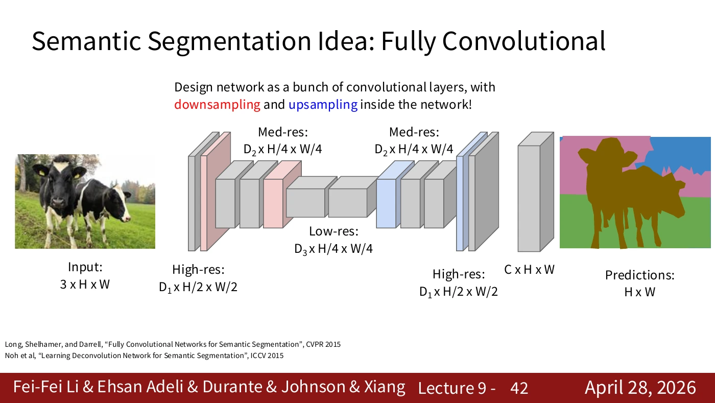
The network processes broad context on a smaller grid, then maps the result back to a dense output. Follow the tensor labels on the slide and the direction in which the spatial dimensions change. Resizing alone cannot recover detail lost earlier.
The original diagram repeats H/4×W/4 at several intermediate points. Treat it as a conceptual view of the two paths. For an implementation, inspect each layer’s actual tensor shape.
#P043. Choosing an upsampling operation
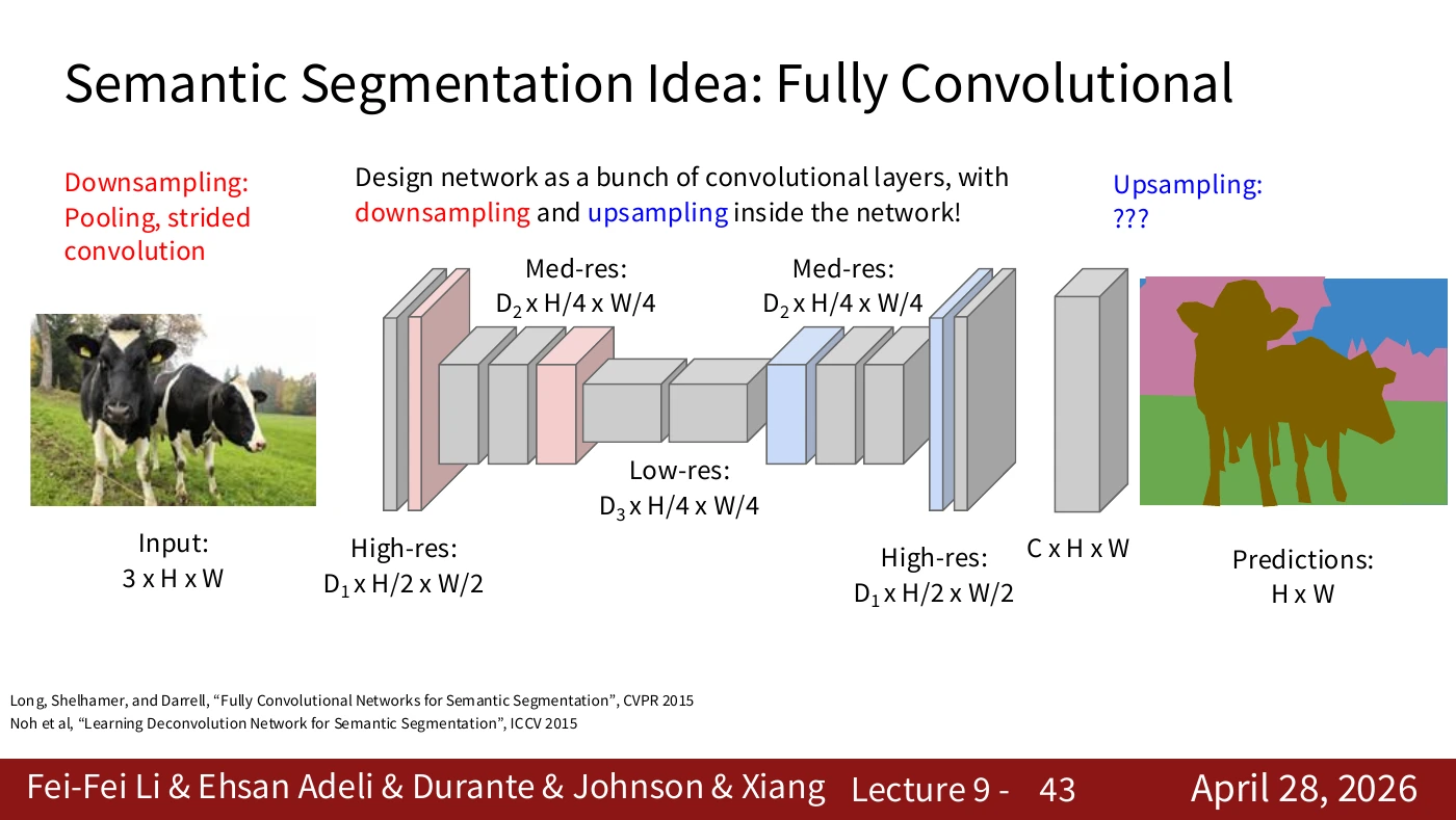
The downsampling path lists pooling and strided convolution. The upsampling path carries a question mark. Unpooling and transposed convolution, introduced next, provide two possible operations at that point.
The paths look symmetric, but they need not be inverses. Enlarging the output cannot reconstruct all the values discarded by averaging or taking a maximum. The arrays on the next two slides show how the expansion rules differ.
#P044. Nearest neighbor and bed of nails
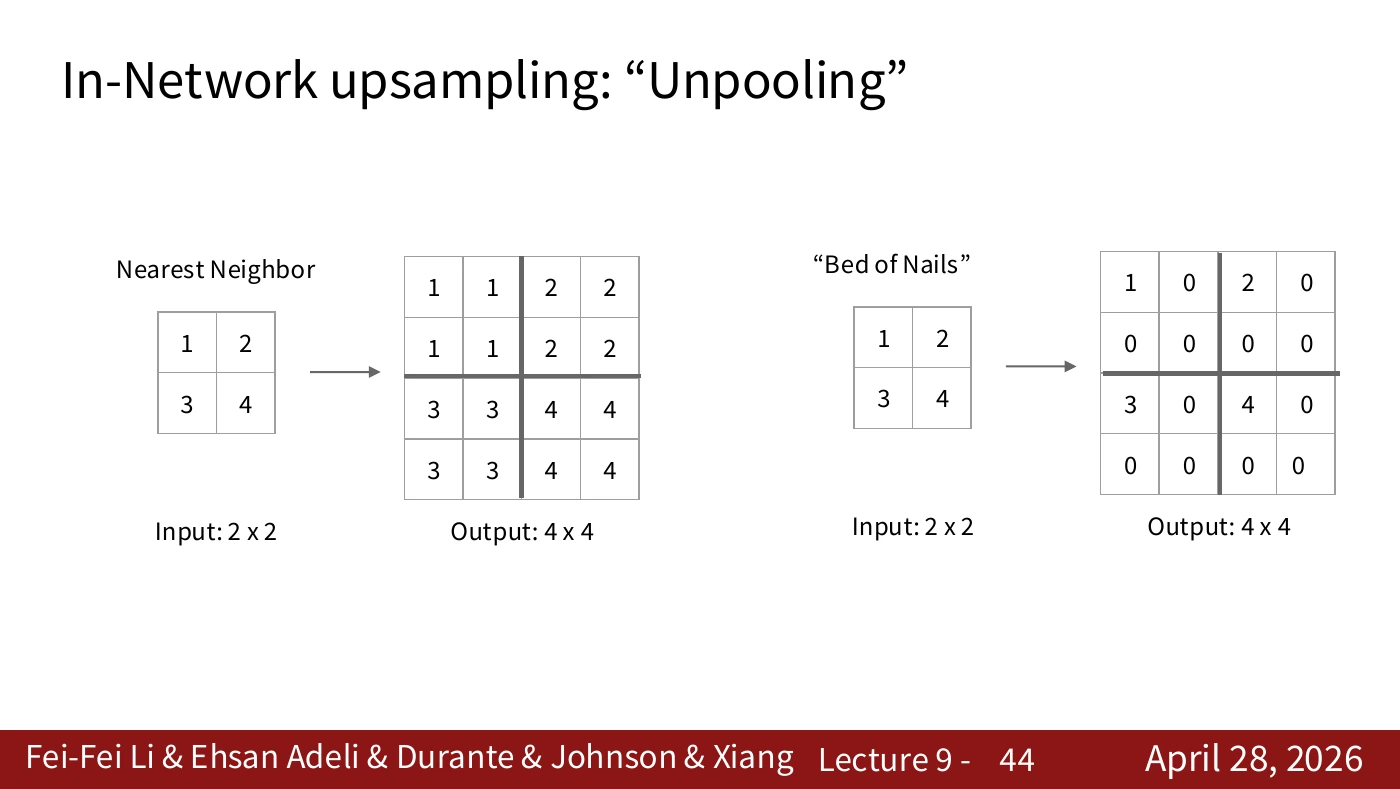
Nearest neighbor copies an input value into several output positions. Bed of nails places the values farther apart and fills the intervening locations with zeros. The output dimensions can be identical while the arrangements of values differ. Neither operation observes a new boundary.
Starting from the slide’s 2×2 input [[1,2],[3,4]], nearest neighbor copies each entry into a 2×2 block. Bed of nails inserts zeros between entries. Both outputs have a 4×4 shape. To check an implementation, inspect the values as well as their dimensions.
#Lecture supplement · Nearest neighbor and bilinear interpolation
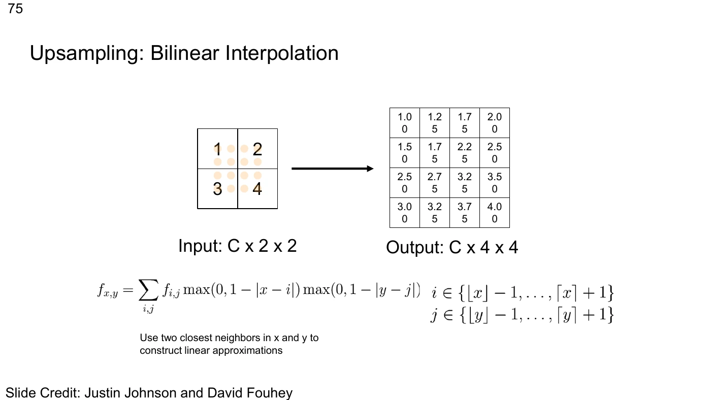
Nearest neighbor on P044 copies the closest value. Bilinear interpolation weights neighbors along both axes according to their distance. Place 1, 2, 3, and 4 at the four corners. At the exact center, each has weight 1/4 and the result is 2.5. At other locations, nearer corners have more weight. The value 2.5 interpolates existing observations. It is not evidence of a new object.
When comparing the 4×4 array with a library result, check which input coordinates correspond to the output pixel centers. Boundary handling and alignment settings such as align_corners can change the intermediate values. The coordinates and weights determine the numerical result.
Interpolation can mix continuous features or per-class scores. Suppose a label map uses arbitrary integers for grass (0), cow (1), and sky (2). A bilinear average of 0.5 has no class meaning. This is why ground-truth masks are commonly resized with nearest neighbor. Model outputs can instead be resized one score channel at a time before taking an argmax.
The 2025 video, 25:13–26:46, covers nearest neighbor, bed of nails, and an operation that stores the location of a maximum. The bilinear example comes from a separate lecture and is included to compare fixed upsampling rules. On P045, ask which locations the network remembers. From P046 onward, ask whether it can also learn the weights of the values sent to those locations.
#P045. Unpooling with saved max-pooling locations
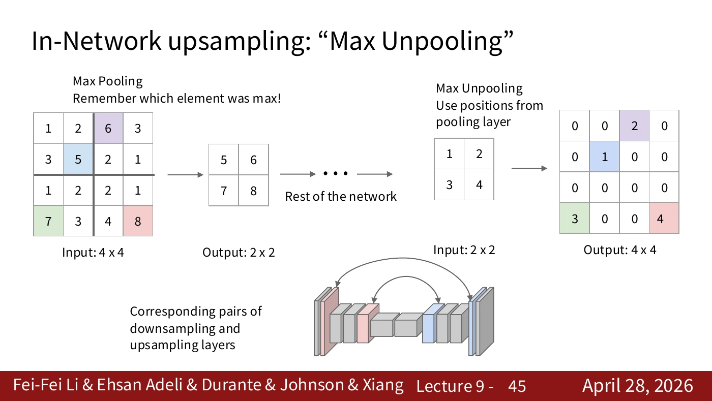
Max pooling can record the location of its selected value. Unpooling places a value at that saved location and fills the other positions with zeros. The encoder and decoder must agree on the corresponding pooling stage. The indices cannot recover every value that preceded pooling.
The figure distinguishes the location saved during max pooling from the value supplied later to unpooling. Even when the value lands at the correct index, the other discarded values remain unknown. The connection under the diagram passes location information between matching stages.
#P046. Starting with the spatial size of an ordinary convolution
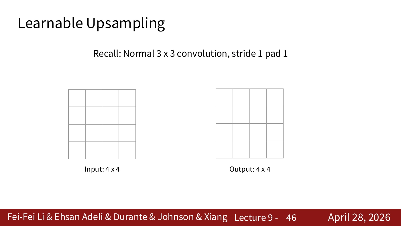
In this example a 3×3 filter operates on a 4×4 input with stride 1 and padding 1. The output remains 4×4. This familiar input–output relationship gives us a reference for the expansion operations ahead.
Kernel size alone does not determine the output shape. Record stride and padding as well. Then you can predict what changes when a setting differs from this 4×4 example.
#P047. One output is a dot product
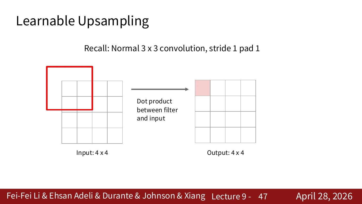
Multiply each filter weight by its corresponding input value and sum the products. This gives one output entry. Identify which input window contributes and where the result is written. The next slide moves the filter and repeats the same operation.
The red window extends beyond the input at its edge. Padding 1 defines the values used at that boundary, so the filter computation follows the specified padding rule.
#P048. Moving the filter and reusing its weights
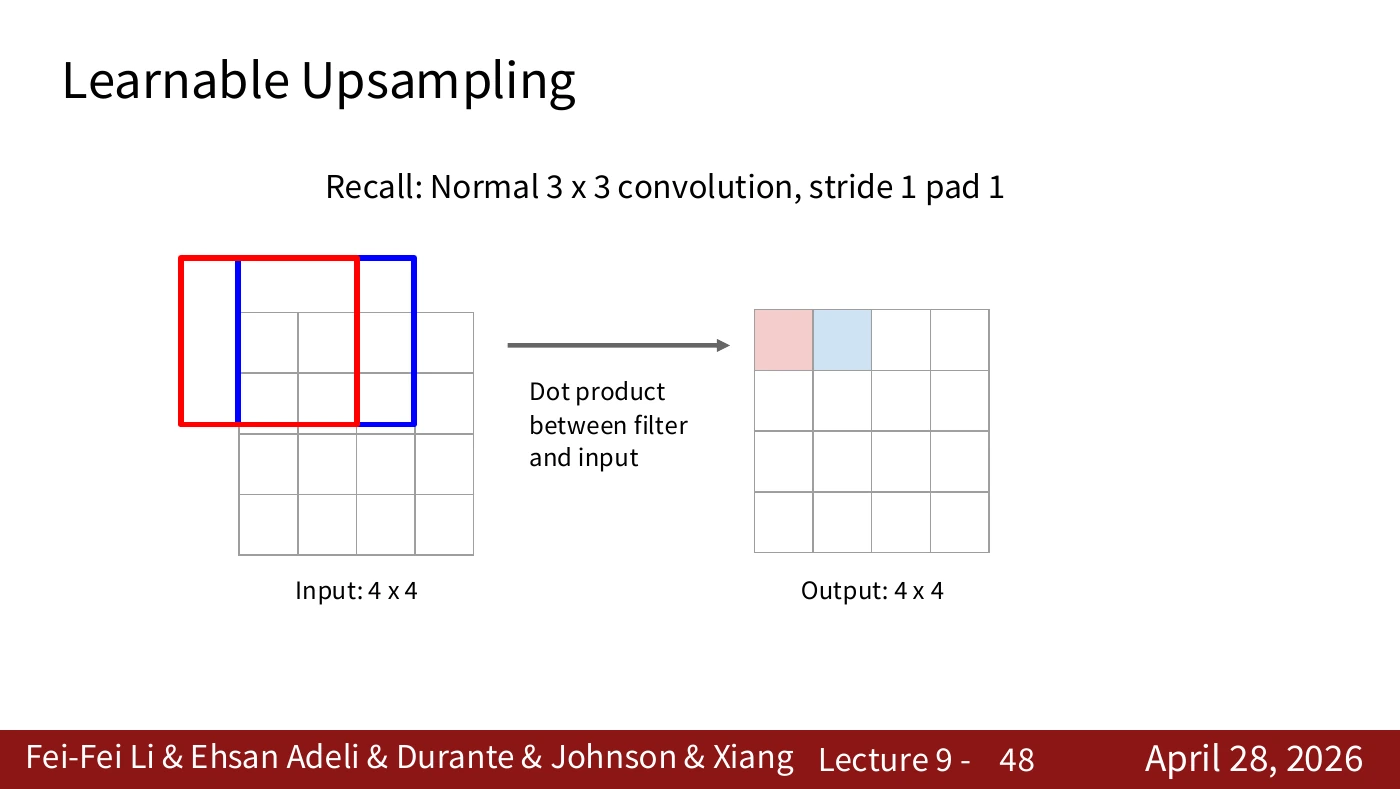
Compare the old and new filter positions. The weights stay the same as the input window changes. Each entry in the output map comes from applying that filter at a different location.
Match the movement from the red window to the blue one with the corresponding red and blue output cells. At stride 1, a one-cell shift in input space corresponds to a one-cell shift in output space. This is what spatial weight sharing looks like.
#P049. Reducing the number of positions with stride 2
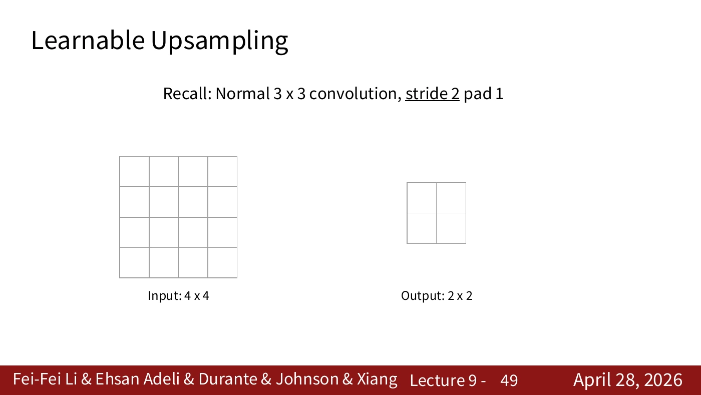
Keep the 3×3 filter and padding 1, but set stride to 2. The output in this example becomes 2×2 because the filter is evaluated at a coarser set of positions. The change concerns spatial resolution. It need not alter the number of channels or categories.
A 4×4 input and 2×2 output mean that four output positions are evaluated. Each filter window still reads several input pixels. Counting output positions alone does not tell you how many input pixels were read.
#P050. The dot product on a coarse output grid
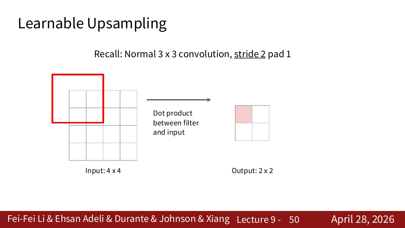
The dot product between filter and input remains the same. What changes is the interval between filter placements. Mark how far the filter moves on the input for one step across the output.
Each output position follows the rule from the stride-1 example. The next window begins at a different offset. Distinguishing the computation from the grid on which it runs makes the transposed operation easier to follow.
#P051. Stride relates movement on two grids
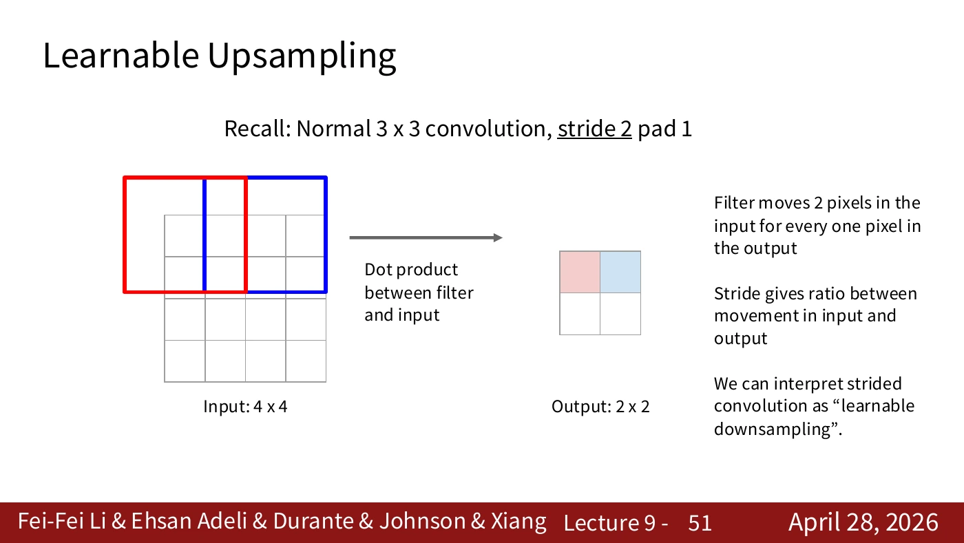
A shift of two cells on the input corresponds to one cell on the output. Strided convolution can therefore learn a downsampling operation. It serves a similar spatial purpose to pooling and has trainable filter weights.
The red and blue windows are two cells apart on the input. Their output cells are neighbors. The next slide reads this spacing relation in the opposite direction. That operation does not require an inverse matrix or guarantee recovery of the original signal.
#P052. Output size in transposed convolution
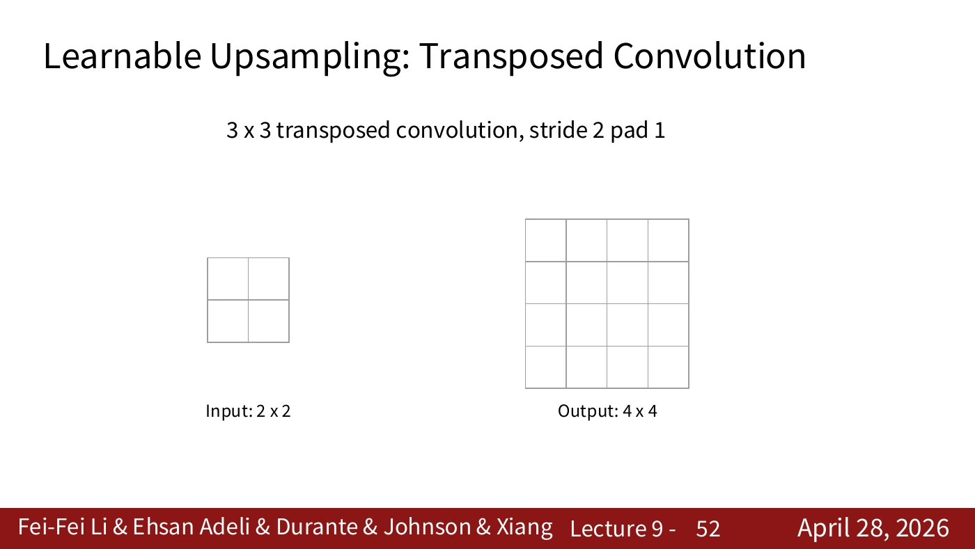
The slide starts with a 2×2 input and constructs a larger output. “Transposed” describes an operator relationship. To reproduce the pictured dimensions in a framework, check its stride, padding, kernel size, and output padding.
For dilation 1, one output dimension is (input_size − 1) × stride − 2 × padding + kernel_size + output_padding. The 2→4 illustration includes a boundary and output-padding choice. For example, with kernel 3, stride 2, padding 1, and PyTorch’s default output padding of 0, an input dimension of 2 gives an output dimension of 3. Match the settings before comparing shapes.
#P053. One input value scales a whole filter pattern
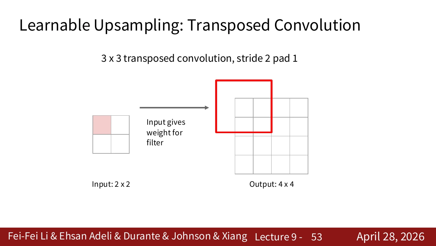
One entry in the smaller input multiplies the entire filter pattern and contributes to a region of the output. Ordinary convolution gathers several inputs into one output. Here it is helpful to track one input as its weighted contributions reach several outputs.
Trace the weights from the red input value into the red 3×3 output region. The filter is shared as its contribution spreads. The enlarged output is computed from the input and weights. It supplies no new ground-truth observation.
#P054. One input step corresponds to two output steps
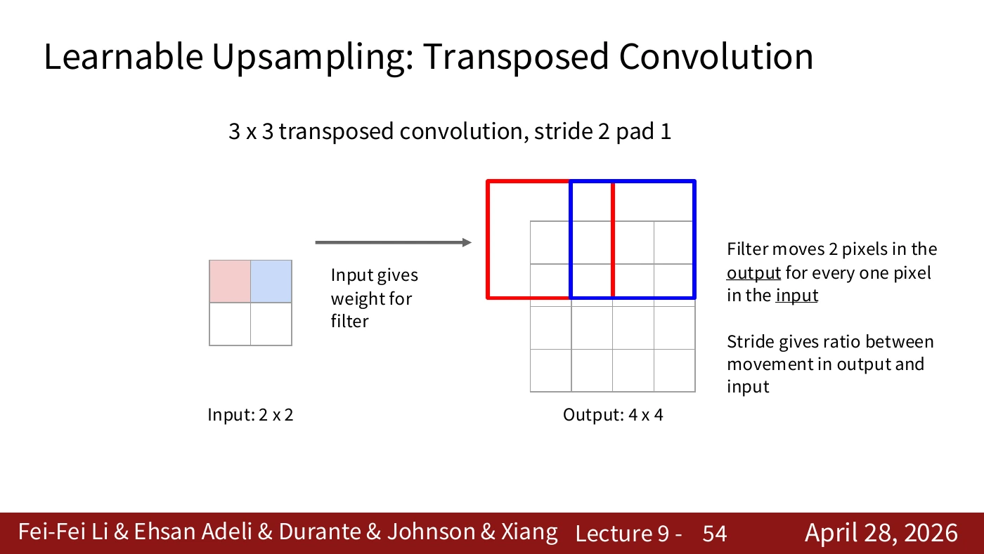
Moving one cell along the input shifts the filter pattern by two cells on the output in this example. Identify the grid on which you measure stride. Neighboring input entries still use the same learned filter.
The red and blue windows begin two output cells apart. The patterns contributed by adjacent inputs can still overlap, as the next slide shows. A larger stride alone does not guarantee a smooth enlargement.
#P055. Adding overlapping contributions
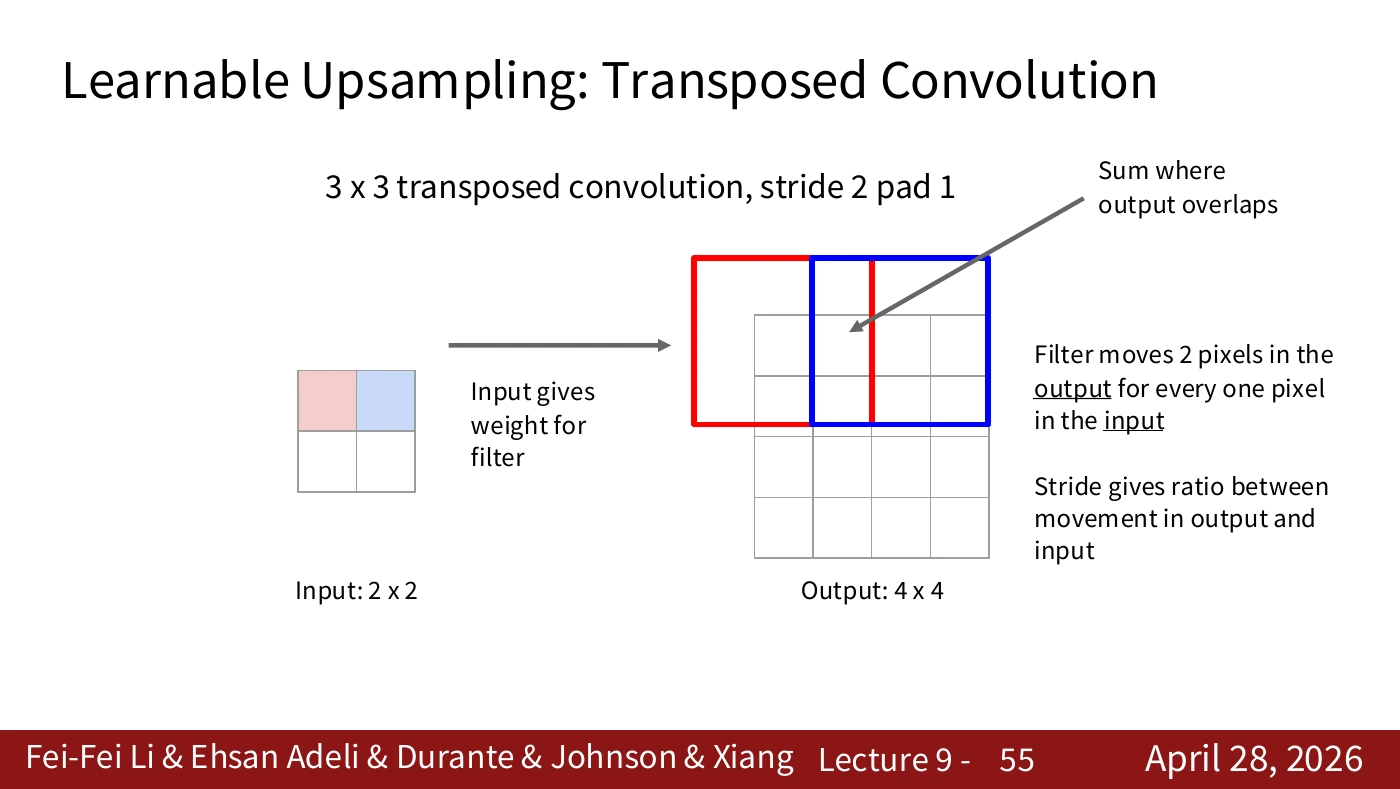
When several inputs contribute to the same output cell, add their values. The later contribution does not overwrite the earlier one. Tracking the number and location of overlaps reveals how this differs from fixed interpolation.
The arrow marks a cell that receives weighted filter values from both inputs. Sum them by hand and compare the result with the implementation. Copying or overwriting would give a different value.
#P056. Summing every input’s contribution
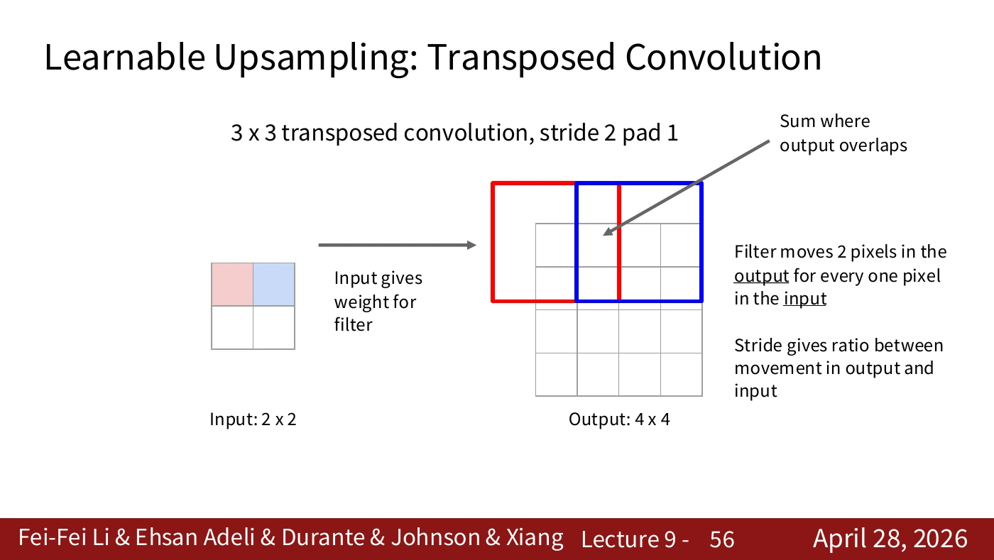
Apply the same overlap rule to the remaining positions. For each output, identify the input values and filter coefficients that contribute to it. The larger grid alone gives no access to the true high-resolution image.
Trace the two colored regions separately, then identify where they overlap. The slide repeats the operation at a new position so that you can see how contributions accumulate across the grid.
#P057. Calculating overlap in one dimension
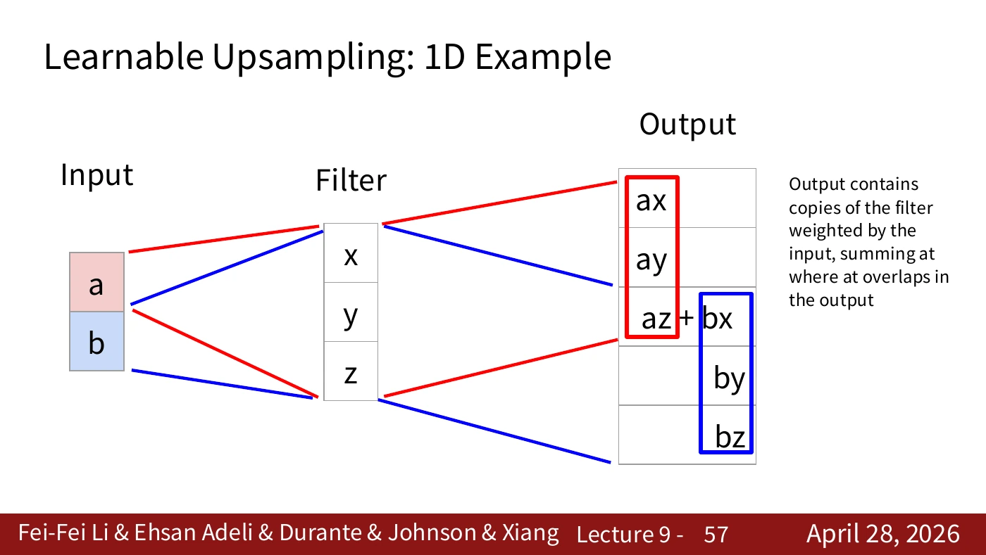
On the slide, a and b are the inputs and x, y, z are the filter. The first input contributes ax, ay, az. Starting two cells later, the second contributes bx, by, bz. Both reach the middle cell, producing az+bx. The output is therefore [ax, ay, az+bx, by, bz]. Check the labels “Input” and “Filter” before assigning the symbols.
Try a=2, b=3, and the filter [x,y,z]=[1,4,5]. The first contribution is [2,8,10,0,0] and the second is [0,0,3,12,15]. Their sum is [2,8,13,12,15]. This worked example was created for the article to illustrate the slide’s rule.
#Video supplement · Why add the overlapping values?
In the 2025 lecture, 28:09–28:46, the instructor expands a and b with a filter and adds the terms that reach the same output location. To read the colors in the larger diagram, write down which inputs reach each output cell.
The terms from a are [ax, ay, az, 0, 0]; those from b, starting two positions later, are [0, 0, bx, by, bz]. Their sum is [ax, ay, az+bx, by, bz]. The center receives contributions from both inputs. The leftmost cell receives only a’s contribution. Uniform copying would miss that difference.
The filter coefficients x, y, z can be learned. Several inputs can have the same downsampled representation, so the enlarged grid cannot uniquely recover information lost during downsampling. This is why the term deconvolution can be misleading: a transposed convolution generally has no claim to be an inverse. P058 places it back in the path that constructs an output map.
#P058. Filling in the network’s upsampling path
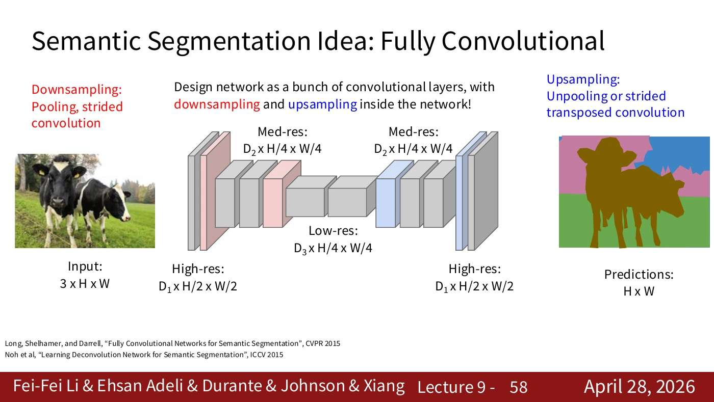
We can now put unpooling or a strided transposed convolution in the upsampling path. The local operations fit into the complete network diagram. To choose between them for a task, compare boundary quality and computational cost in an experiment.
Label the downsampling and upsampling operations, the intermediate feature channels, and the final class score map separately. Network depth does not set the number of final categories. That number comes from the dataset’s label scheme.
#P059. Reading the U-Net architecture
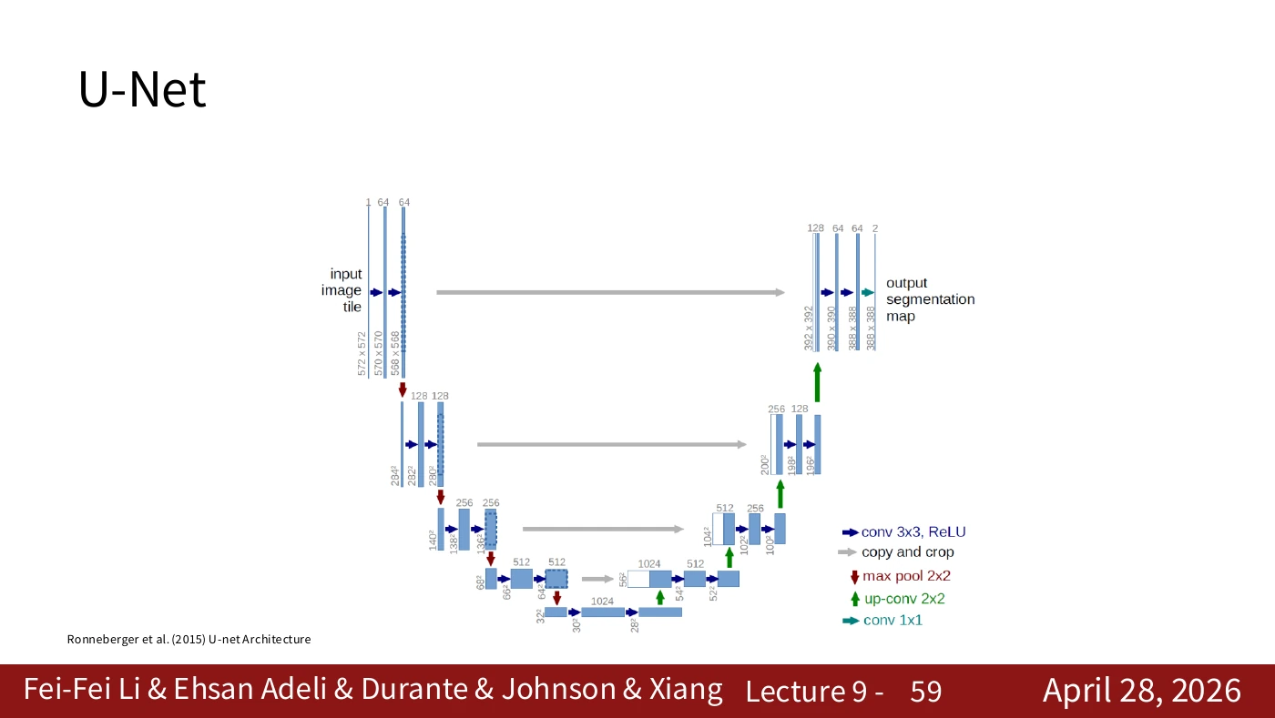
Identify the descending path, the ascending path, and the connections between them. The original U-Net comes from the 2015 paper by Ronneberger and colleagues. Trace the changes of resolution and the skip connections in that diagram. Later implementations can follow different sizing rules.
Distinguish the blue boxes and horizontal links from the downward and upward arrows. The original network uses valid convolution and cropping, so input and output have different dimensions. An implementation with same padding may have different shapes.
#P060. The descending path gathers wider context
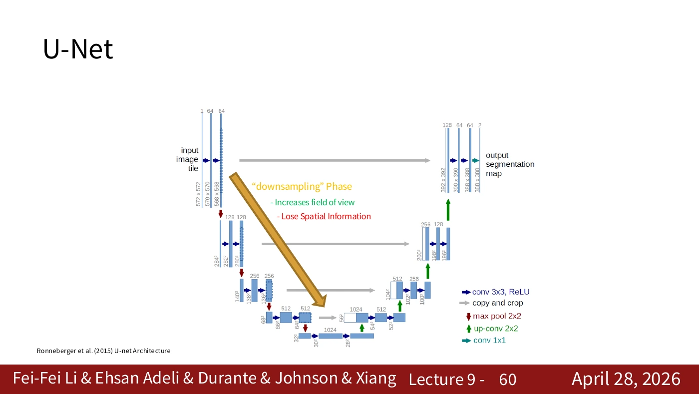
Downsampling combines information from a wider area while fine positional detail becomes less directly available. Identifying that loss explains why the next path is needed. Deep features alone can struggle to preserve thin boundaries.
Farther down the path, features can incorporate a larger input region. Meanwhile, a small boundary’s exact location may become less explicit. Recognizing what is present and locating its boundary precisely are distinct requirements.
#P061. The ascending path builds a dense map
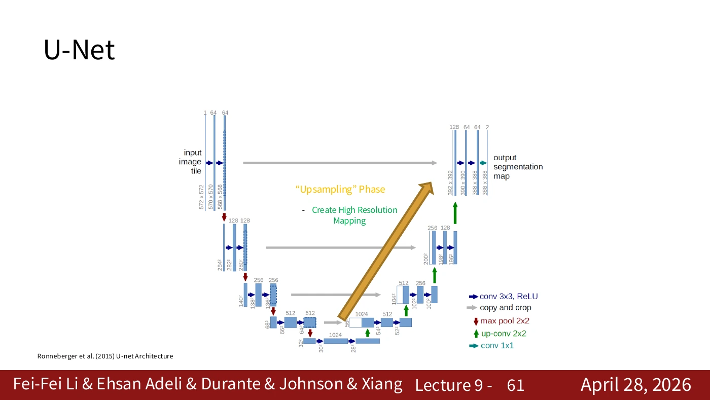
Upsampling yields a denser set of output positions. Having more positions does not by itself determine the correct boundaries. The next slide introduces a connection to higher-resolution features that helps restore spatial detail.
Follow the ascending path as it constructs the dense map. For a detailed boundary near the top of the diagram, the network can integrate information from the earlier path. This additional input distinguishes U-Net from a simple image resizer.
#P062. Concatenating high-resolution features
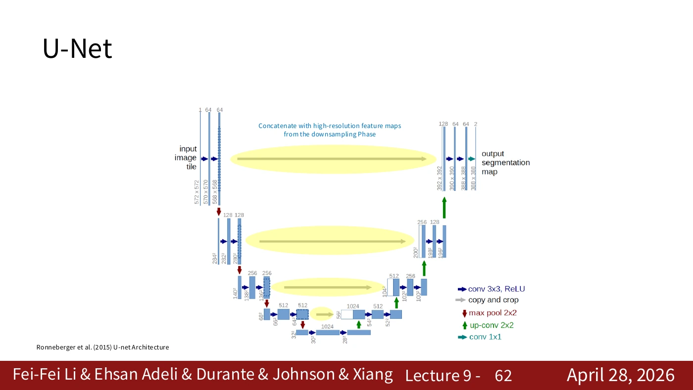
U-Net concatenates features from the descending path with features on the ascending path along the channel axis. FCN’s addition of class scores uses a different operation. The spatial grids still need to align. Modern AI VI examines the original paper’s crop and shape calculations in more detail.
The horizontal connection is labeled “copy and crop” in the original diagram. Addition requires matching channel counts and combines corresponding entries. Concatenation stacks the channels, after which a convolution processes the combined features.
#Paper supplement · Reading U-Net’s arrows as copy and concatenate
Place section 2 and figure 1 of the U-Net paper beside P059–P062 and follow a horizontal arrow. The left path gathers context as resolution falls. The right path increases resolution for location-specific predictions. Enlarging a feature map alone cannot retrieve a thin cell boundary or small structure. The horizontal arrow carries finer features from the left to the corresponding resolution on the right.
The original network uses channel-wise concatenation. For a worked example in H×W×C order, combine two 64×64×32 tensors. The spatial shape stays 64×64 and the channel count becomes 64. A following convolution learns which combinations to use. These dimensions illustrate the operation; they are not the actual channel counts in the paper’s figure. FCN fusion and U-Net concatenation are both skip connections, but they combine different quantities in different ways.
Cropping in copy and crop performs a specific job. Convolution without padding shrinks the original U-Net’s feature maps at the edges. Cropping makes the spatial dimensions compatible for concatenation. Modern implementations with same padding may have different input and output dimensions or cropping requirements. Check each tensor in the running implementation against the corresponding arrow.
The 2025 video, 29:11–31:17, also explains why spatial information travels from encoder to decoder. The paper discusses augmentation and training when annotations are scarce. The architecture alone does not guarantee strong performance in that setting. Ask which features at which resolution are combined, and by what operation.
#P063. Tracing the three computation paths
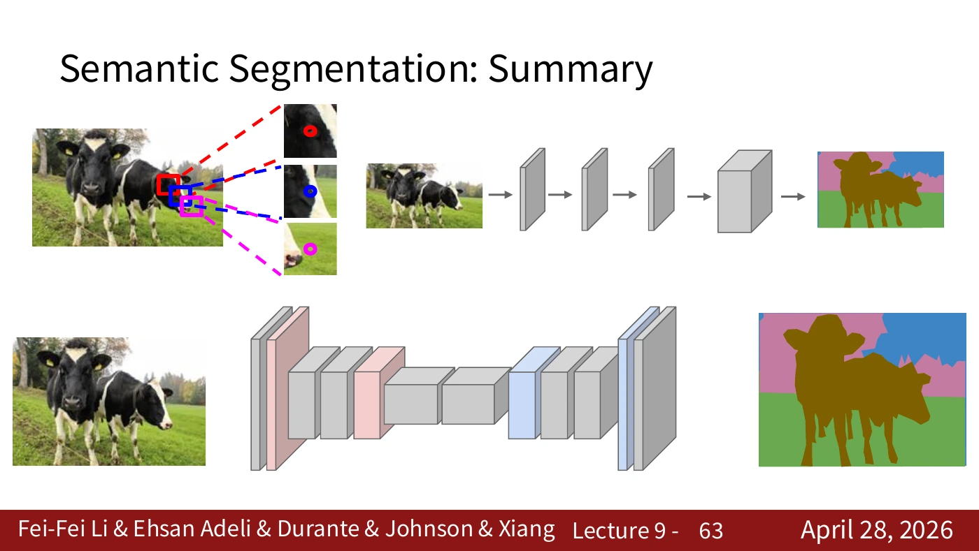
The top diagram repeats a CNN on overlapping patches. The middle diagram shares features at full resolution. The bottom diagram reduces resolution internally and then increases it. Each solves the same pixel-classification task. First, spatial context becomes available through patches. Next, sharing avoids duplicate work. Finally, processing a smaller grid addresses the cost of full-resolution computation.
Compare the identical output requirement with the different intermediate computations. The diagram does not rank their performance across datasets. Measure accuracy, boundary quality, speed, and memory under comparable conditions.
#P064. Semantic labels and individual objects
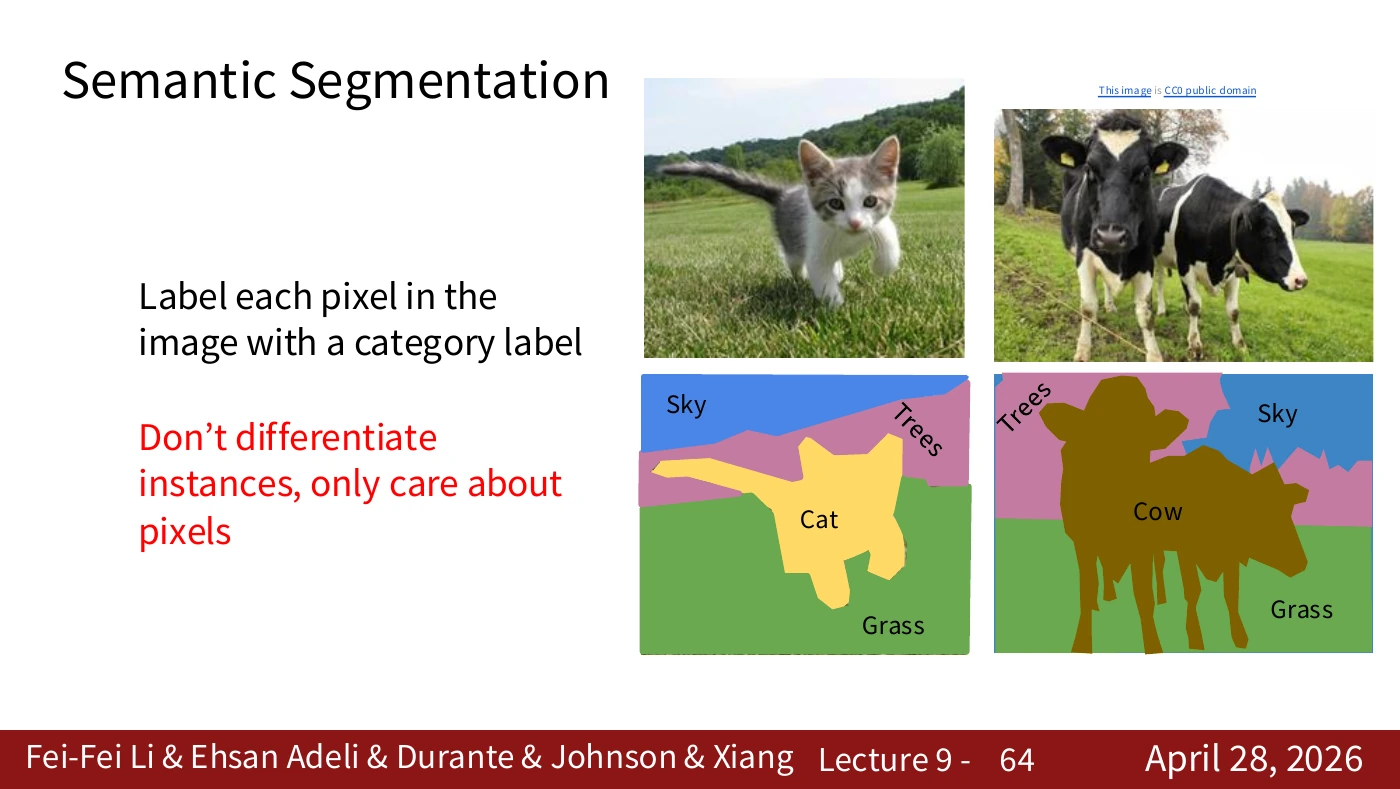
Each pixel receives a category, but two objects in the same category receive the same label. A class such as sky, grass, or animal carries different information from the identity of an individual animal. The CC0 mark on part of the figure concerns that item and does not by itself license the entire slide.
Even if two cows are present, both receive the cow label in the category map. Choosing a single target for manipulation may require an additional way to separate instances. With that distinction in mind, we can return to segmentation as an observation for reinforcement learning.
#Worked calculation · Scores, class IDs, and training loss
In the notation below, z is a real-valued model score, c a class, and (h,w) an output position. These quantities have no physical units.
Training does not minimize the numerical difference between predicted and true IDs. Assigning the cup class ID 7 instead of 1 does not change its meaning. A common approach converts class scores to probabilities with softmax and uses cross-entropy with the true labels. The following standard illustrative objective averages the loss over all valid positions. It is an example for this article.
Ω is the nonempty set of valid labeled pixels. y identifies the true class, and p supplies its predicted probability at that location. A true-class probability of 0.8 gives a loss of about 0.223. At 0.2, the loss is about 1.609. Confidently predicting a wrong class increases the loss. Implementations typically use a numerically stable function on logits and separately specify ignored labels, class weights, and the reduction rule.
#Worked example · Checking mask IoU by hand
This small, dependency-free Python example evaluates two masks without training a model. The cup masks were chosen to have an intersection of 6 pixels and a union of 12.
prediction = {0, 1, 2, 3, 4, 5, 6, 7, 8}
ground_truth = {3, 4, 5, 6, 7, 8, 9, 10, 11}
intersection = len(prediction & ground_truth)
union = len(prediction | ground_truth)
iou = intersection / union if union else None
print(intersection, union, iou)  # 6 12 0.5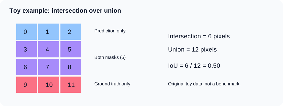
A 12-pixel grid drawn for this article. Blue marks prediction-only pixels 0–2, purple marks shared pixels 3–8, and pink marks ground-truth-only pixels 9–11.
P is the predicted region and G is the ground-truth region. Their sizes are pixel counts, and the ratio is dimensionless. If both are empty, the denominator is zero. The example returns None to expose the case. Each benchmark specifies its convention. Before averaging IoU over classes, check which classes count, how empty classes are handled, and how scores are aggregated across the dataset.
Pixel accuracy can favor a model that correctly labels a dominant background. Missing every pixel of a small cup can still leave high overall accuracy. Conversely, a mask with high IoU can miss a small boundary where the gripper makes contact and cause a failed grasp. Measure perception quality and task success separately.
#Lecture supplement · A high IoU may not transfer to another camera
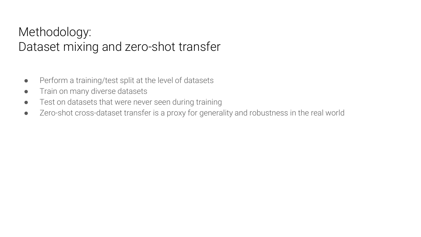
The preceding IoU example compares a prediction and a reference on the same pixel grid. The choice of evaluation data is another question. The supplementary slide trains on multiple datasets and evaluates on a dataset held out from training. Randomly splitting adjacent frames from one video can put nearly identical scenes on both sides. In that situation, the score may measure recognition of a familiar scene while saying little about a new location.
Imagine moving a model that segments cups on a brightly lit desk to a camera in a dim corridor. Lighting, background, camera height, and occlusion can all change the input distribution even when the target is still a cup. Mixing datasets can expose the model to some of that diversity. It also requires reconciling category names and boundary-annotation rules across datasets.
Here zero-shot cross-dataset transfer means evaluation on a dataset that the model did not use for training. In this setting the phrase does not claim support for arbitrary new categories specified by a text prompt. The lecture treats the evaluation as a proxy for generalization and robustness in the real world. Evidence for a particular deployment still requires observations from that setting.
Before using the class mask from P064 as a robot observation, record whether test scenes are independent of training scenes, whether the camera or preprocessing changed, and whether the mean conceals errors on small targets. Mean IoU and physical task success measure different outcomes.
#Back to the robot · What follows the mask?
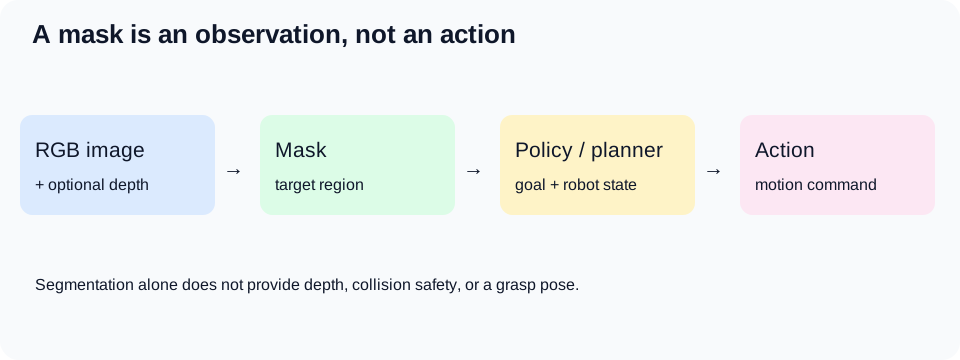
An illustrative system diagram drawn for this article. Other robot systems and papers use different architectures.
A cup mask lets you collect foreground pixels or select cup points in a depth image. A mask alone cannot tell you the 3D position, hidden surfaces, mass, or chance that the gripper will slip. When using depth, also check the camera calibration and coordinate transformation.
At minimum, record the following separately in a robot experiment.
- Perception. Does the mask remain stable for small, occluded, or reflective objects?
- Timing. What is the latency from camera input to the output used by the controller?
- Geometry. Are depth and mask aligned in time and coordinate frame?
- Action. Does grasping fail even when the mask is correct? Is collision checking performed separately?
A policy can learn directly from raw images or use masks or features as inputs. A strong segmentation model alone does not establish a strong RL policy. Changing a perception output changes the policy’s observation distribution. Differences in preprocessing, resolution, or latency between training and execution also change the conditions at the policy input.
#Watching the video with the transcript
For the original Korean article, the author checked the manually prepared English captions (en-US), comprising 1,173 segments, for the official Stanford Online recording on November 12, 2026. The listening guide below summarizes the relevant spoken passages. Technical terms can be transcribed imperfectly even in a manual caption track. Use the video’s captions or transcript for the exact wording.
Matching the two editions. The links give start times from the 2025 caption track, rounded down to whole seconds. The right-hand column lists pages to read alongside each topic in the 2026 PDF. Around 31:42, the lecturer explains that some slides were placed later in the deck, so the recording cannot be assumed to use the same order or slide transitions.
| Start in the video | Topic confirmed in the captions | Read alongside it in the 2026 material |
|---|---|---|
| 17:45 | Semantic segmentation assigns a category to every pixel in an image. | P032–P033 |
| 18:26 | One pixel lacks context. A surrounding patch provides it, but running the entire network at each position repeats work. | P034–P038 |
| 20:57 | A fully convolutional network computes a spatial output map over the image. | P039–P041 |
| 21:40 | The network lowers spatial resolution for processing and raises it again for the output. | P042–P043 |
| 24:04 | The training objective combines losses from pixel-level classification. Supervised training requires ground-truth label maps. | Worked calculation on softmax and loss |
| 25:13 | Nearest neighbor, bed of nails, and unpooling with saved maximum locations use different rules. | P044–P045 |
| 26:46 | Upsampling can use learned weights. Contributions that reach the same cell are added. | P046–P056 |
| 28:09 | A one-dimensional example with inputs a and b shows each filtered output and the sum where they overlap. | P057 |
| 29:11 | U-Net combines downsampling, upsampling, and features carried from encoder to decoder. | P059–P062 |
| 32:40 | Pixel categories alone cannot distinguish two objects of the same class. | P063–P064 |
| 33:07 | The recording moves to instance segmentation after the semantic segmentation unit. | Beyond this article’s slide commentary |
Read the video’s discussion of ground-truth maps in the context of supervised segmentation. Tools can help create labels while the learning objective still requires a supervision signal. The other distinction to retain is that a transposed convolution learns an expansion operation. It cannot generally invert a loss of information.
The following short presentation script was written for this lesson and expresses the ideas in the author’s own words.
Knowing that a cup is present leaves a practical question: which pixels belong to it? Semantic segmentation gives a category to every position. Instance segmentation can separate individual cups. The model computes several class scores at each position and selects the largest. Reducing resolution saves computation, but enlarging a grid cannot by itself recover the lost boundaries. Follow the architecture to see how it preserves context and location together. A robot can use the resulting mask as an observation. It still needs to handle depth, coordinate frames, collision checks, and the policy that chooses an action.
#A reading order for the supplementary material
- FCN paper. After P039–P043, read section 3 on convolutionalization and upsampling and section 4.2 on skip fusion. They explain how a classifier becomes a pixel predictor and why its boundaries can initially be coarse.
- U-Net paper. Start with figure 1 and section 2 to identify what travels across the horizontal arrows on P059–P062. Compare cropping, concatenation, and output resolution with the implementation.
- Georgia Tech Lecture 14. The full deck begins with background on VGG, Inception, and ResNet. This lesson uses the FCN figure on PDF p. 57, bilinear interpolation on p. 70, and dataset transfer on p. 90. The PPTX is editable. Public access to the file does not itself grant free reuse of every image it contains.
- 2025 Stanford video. Use the timestamps to revisit operations that were difficult to follow in the text or figures. Follow concepts across the two editions without assuming a one-to-one mapping to the 2026 slide numbers.
- Modern AI VI. Continue from pixel-level classification, FCN, and U-Net to the architectures and papers discussed in the existing advanced article. Its role is follow-up reading alongside the slides used here.
#Sources and related reading
- Stanford CS231n, 2026 Lecture 9, April 28, 2026. This article covers PDF pp. 32–64. Each slide links to its source page. The original was checked on November 12, 2026.
- Stanford Online, CS231n Spring 2025 Lecture 9. Supplementary video from a different year. The author checked the manual English captions and spoken timestamps for the semantic segmentation section. The links identify topics in the video.
- Long, Shelhamer, Darrell, FCN, CVPR 2015 · Ronneberger et al., U-Net, 2015.
- Editable lecture material: Georgia Tech CS6476 Fall 2025, Lecture 14 PPTX / PDF. Numbered P-sections in this article refer to the Stanford PDF.
- Advanced reading: Modern AI VI · Starting point: Robot Learning 01.
The original slides are cited for study and discussion of the material they illustrate. Rights remain with their authors and the owners of the individual images. This article grants no reuse license for those materials. Author credits and page numbers are preserved. The full lecture PDF is available at its original source. The author used AI assistance for the original Korean commentary, additional numerical examples, presentation script, and supplementary diagrams.