When we watch a robot pick up a cup, can we tell what it has learned? Let us follow the information it sees, the actions it chooses and the signals it learns from to build a picture of robot learning.
Lecture video · Oier Mees, ETH Zurich 2026 · Official course · Slide PDF
#P001 · What does a robot learn?
Robot learning is the broad field of applying learning methods to problems in robotics. Reinforcement learning (RL) is a way to improve decisions using the consequences of actions and the rewards they produce. The presence of an AI model in a robot does not mean that the robot was trained with reinforcement learning.
Imagine a robot moving a cup. A model that locates the cup in an image, a model that predicts how far it will move when pushed, and a policy that decides which way to move the gripper each have a different job.
| Question | What we learn or design | Role |
|---|---|---|
| Where is the cup? | Perception or representation model | Extract information needed for action from an image. |
| How will it move if pushed? | Dynamics model | Predict what changes after an action. |
| What should I do now? | Policy | Choose an action from the observation and goal. |
A policy can learn from human demonstrations or improve through rewards. This chapter maps the field by separating a robot’s inputs, actions and learning signals.
#P003 · Oier Mees and robot learning research
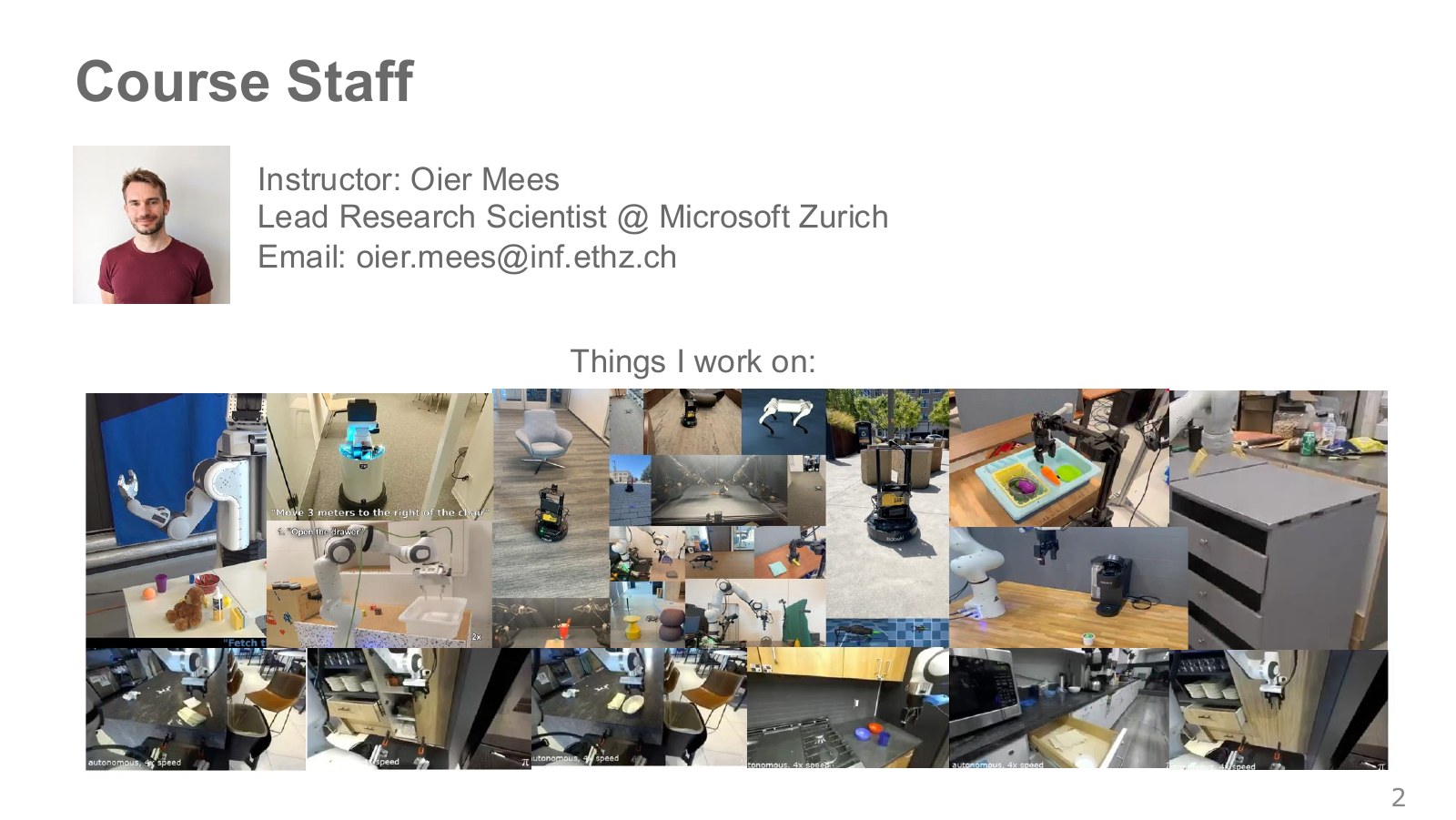
The lecturer, Oier Mees, earned his PhD in Freiburg, worked with Sergey Levine at UC Berkeley, and then moved to Zurich. The research collage on the slide spans manipulation with robot arms, mobile robot navigation, quadrupeds and drones. The course explores the principles of imitation and reinforcement learning that connect these tasks.
Marc Pollefeys introduced the background linking ETH’s Department of Computer Science with Microsoft’s spatial AI research. In the collage, Mees pointed to a Google robot opening a drawer as a real application of algorithms the students would learn.
At the time of the lecture, Mees was a Lead Research Scientist at Microsoft Zurich. His current work and affiliations are listed on his personal website, which also records his move to Project Prometheus in August 2026.
- Lecturer: Oier Mees · Contact listed in the course materials: oier.mees@inf.ethz.ch
- ETH lab: Computer Vision and Geometry Group
- Course mentor: Marc Pollefeys · marc.pollefeys@inf.ethz.ch
- Microsoft lab introduced in the lecture: Spatial AI Lab, Zurich
- Related lab: Berkeley Robot Learning Lab
Following these researchers’ papers and projects reveals how the same policy-learning ideas carry across different hardware and tasks.
#P007 · Understanding foundations, practice, models and systems together
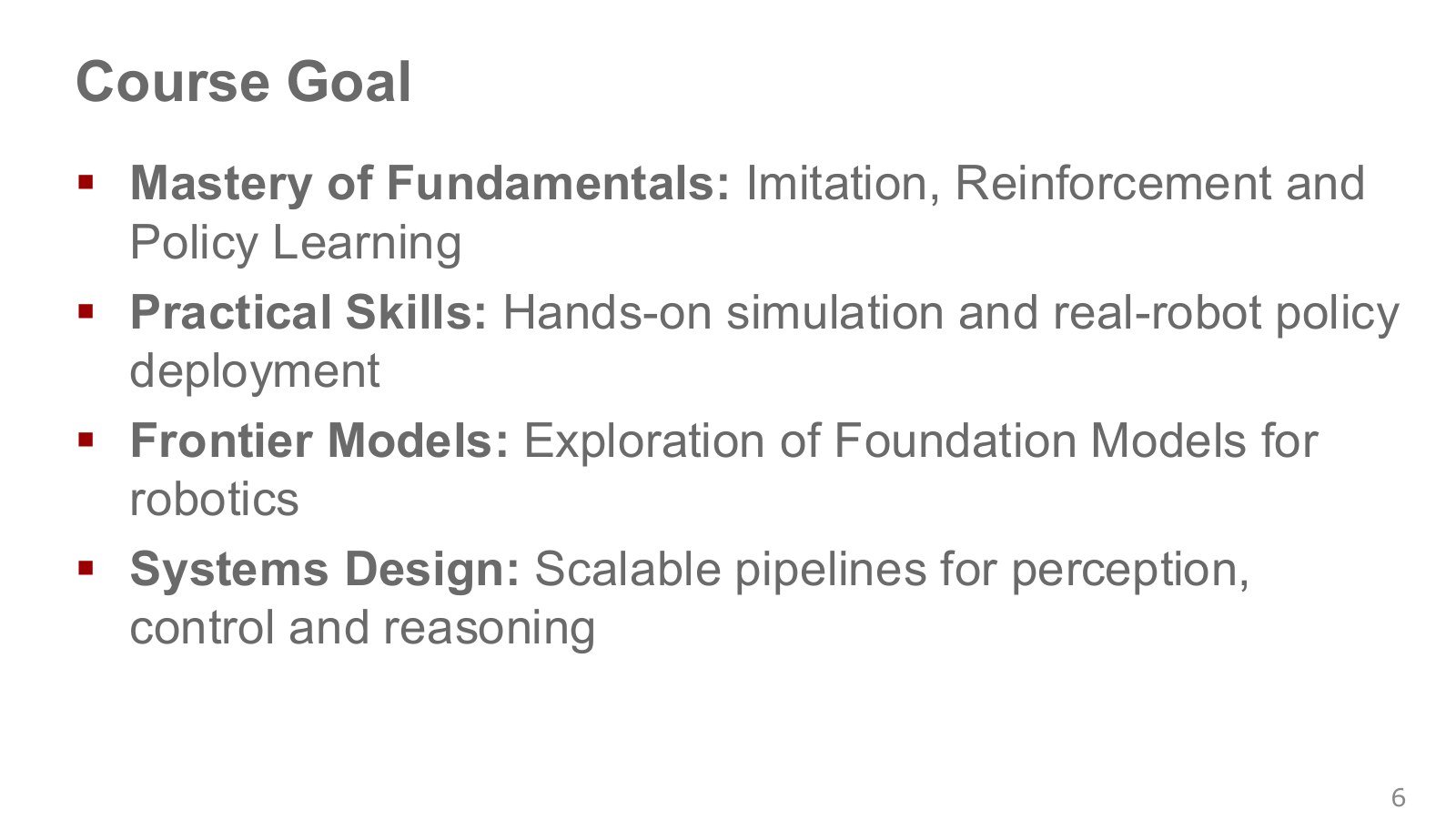
Robot learning extends beyond training a large neural network. We need to understand the underlying algorithms, implement them in simulation, connect them to real robots, and make perception, control and reasoning work together.
A policy is a rule for choosing an action from the information available. It takes camera images, joint positions and task instructions, then chooses the next command. Think of action = policy(observation, goal). Executing a policy means computing actions with that rule; learning a policy means changing the rule in response to data and an objective.
| Four course goals | A question to keep in mind |
|---|---|
| Foundations of imitation learning, reinforcement learning and policy learning | What signal improves the behavior? |
| Practice in simulation and on real robots | How do observations and actions connect to code? |
| Robot foundation models | How is knowledge shared across tasks? |
| Systems linking perception, control and reasoning | How does a model’s output become physical movement? |
Even when a model chooses the right direction, mismatched coordinate frames, units or command timing can send the robot somewhere unintended. That is why the model and its execution system need to be studied together.
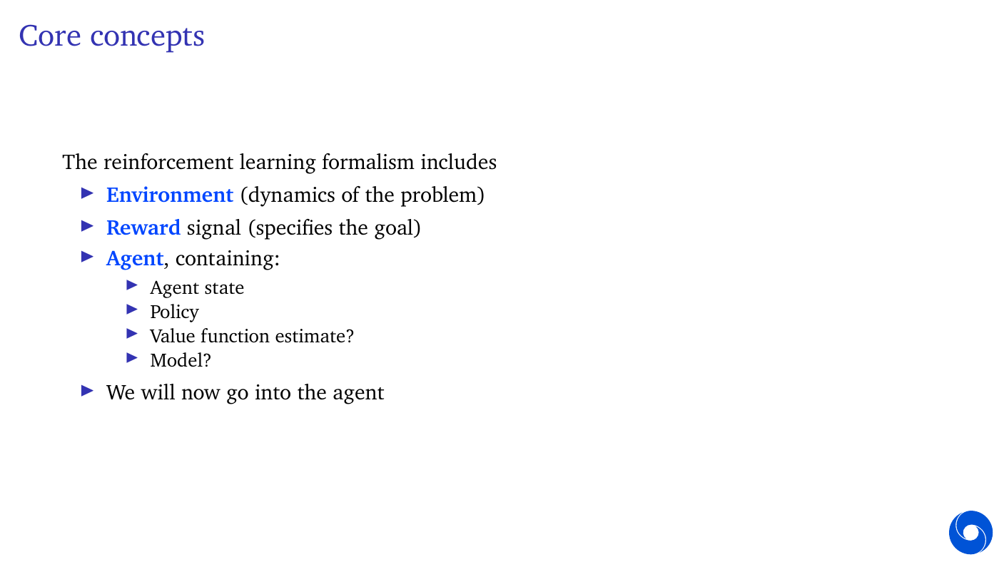
DeepMind/UCL Lecture 1, 33:59–36:21 distinguishes policies, value functions and environment models. A policy chooses actions, a value function estimates the sum of future rewards, and an environment model predicts what changes after an action. In the cup example, the policy decides whether to push right, the value assesses how much that choice helps with the eventual tidying task, and the model predicts where the cup will end up. An agent need not learn all three. A random action rule is still a policy, and some policies operate without a value function or a learned environment model.
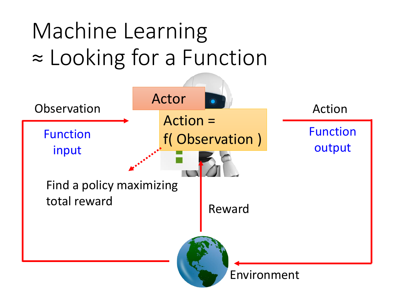
The Actor in NTU’s introductory lecture, 5:00–6:28 can be understood from the same starting point: a function that receives an observation and produces an action. When different lectures use different terms, first match their inputs and outputs. The object we want to learn here is a rule for behavior that repeatedly interacts with an environment, rather than a single correct answer.
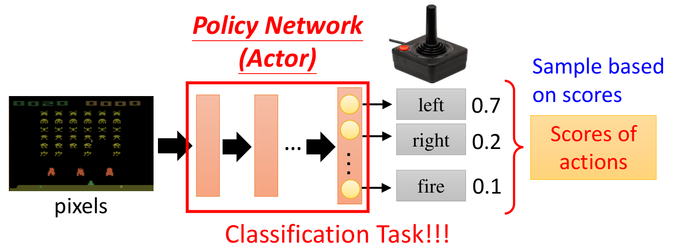
Read the figure from left to right: screen pixels, a neural network to be trained, then possible actions and their probabilities. The value 0.7 means the probability of choosing left on the current screen; it does not mean that moving left earns a reward of 0.7. The NTU video, 13:27–15:24 also starts with an input/output structure resembling a classification network. But supplying the correct label “cat” in classification and improving a policy through the long-term consequences of actions involve different learning signals.
We can express this stochastic choice using observation-based notation. The equation below explains the diagram, with its screen input written as the observation .
Explore the symbols and calculation Choose action from the distribution specified by policy for observation
Read the equation in words
Feed the robot's current view into the policy, then sample one action from its distribution. The same observation can permit several actions.
Understand each symbol
- The sensor observation at step . It is not assumed to equal the full physical state.
- The action chosen at step : for example, a torque, a joint target or a movement direction, depending on the setup.
- A policy that maps an observation to an action distribution. The subscript denotes the weights that define it.
- The parameters collecting the trainable weights of the network or policy.
- The index of a step at which the robot acts in the environment, distinct from elapsed time in seconds.
- Conditional notation: the information to the right of the bar is given. This is not a division sign.
Follow the calculation
- Supply the sensor observation.
- Compute the probability assigned to each action, then choose one according to those probabilities.
Check with a small example
With probabilities of 0.7 for left and 0.3 for right, repeated choices approach about 70% left; ten choices need not contain exactly seven left actions.
An illustrative example for understanding the equation.
is the step at which an action is chosen, is the observation at that step, is the selected action, and represents the network’s trainable parameters. means sampling from a distribution. Sampling 100 times on the same screen does not guarantee exactly 70 left actions, although the proportion approaches 0.7 over many repetitions. Always choosing the action with the largest value is another execution rule, distinct from sampling. For continuous robot-arm commands, we might model a distribution over displacements or joint targets instead of three buttons.
The course sequence reflects these four goals. Students begin with core algorithms, present and critique papers, write simulation code for individual assignments, and then move to a group project with a real robot. In the 2026 course, paper presentations and discussion accounted for 20%, coding assignments for 40%, and the group project for 40%; there was no separate final exam. This is an example of the course organization at that time, not current enrollment guidance. It explains why these notes connect theory, papers, implementation and evaluation on real hardware. The four individual assignments and the teams for paper presentations were distinct from the real-robot project teams.
The lecturer urged students to start assignments early because getting code to run is only the beginning of training. They need to wait for convergence, and a mistake in observation normalization or action units can require another training run after correction. Even in a small simulator, recording data generation, training and rollout evaluation separately helps distinguish “the code runs” from “the robot learned a behavior.” Official course structure
#P008 · Will robotics have its own “ChatGPT moment”?
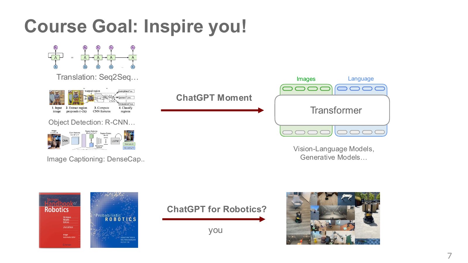
Translation, object detection and image captioning used to rely on separate models. Advances in Transformers and large-scale pretraining shifted the field toward sharing representations and knowledge across tasks. The slide asks whether a similar shift is possible in robotics.
Vision-language-action models (VLAs) aim to connect knowledge from language and vision models to robot actions. RT-2, for example, represents robot actions as tokens and fine-tunes a model on both robot trajectories and vision-language data. At execution time, the output tokens are converted back into robot actions.
Here, Transformer describes the architecture, VLA describes the kinds of inputs and outputs, and reinforcement learning describes a training method. The same Transformer architecture can learn from demonstrations or improve through rewards. Keeping three questions separate—what information goes in, what comes out, and what signal trained it—makes model names easier to interpret.
#P015 · From robots on screen to real research questions
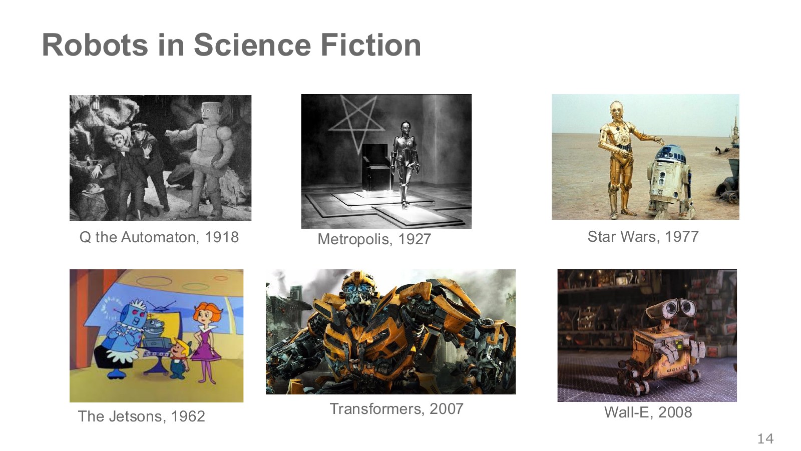
Film and animation have long shaped our expectations of robots. The imagined roles have expanded from machines that take over factory work to household helpers and characters that form relationships with people. The slide places Metropolis, The Jetsons, Star Wars, Transformers and WALL·E side by side.
To turn those expectations into research questions, we need to break “working like a person” into smaller actions. Finding a cup, reaching for it, gripping it without slipping, carrying it around obstacles and placing it at a target each pose different problems. Even a movement that looks natural to us requires a robot to connect perception, planning, contact and control.
#P016 · Why do we need robots?
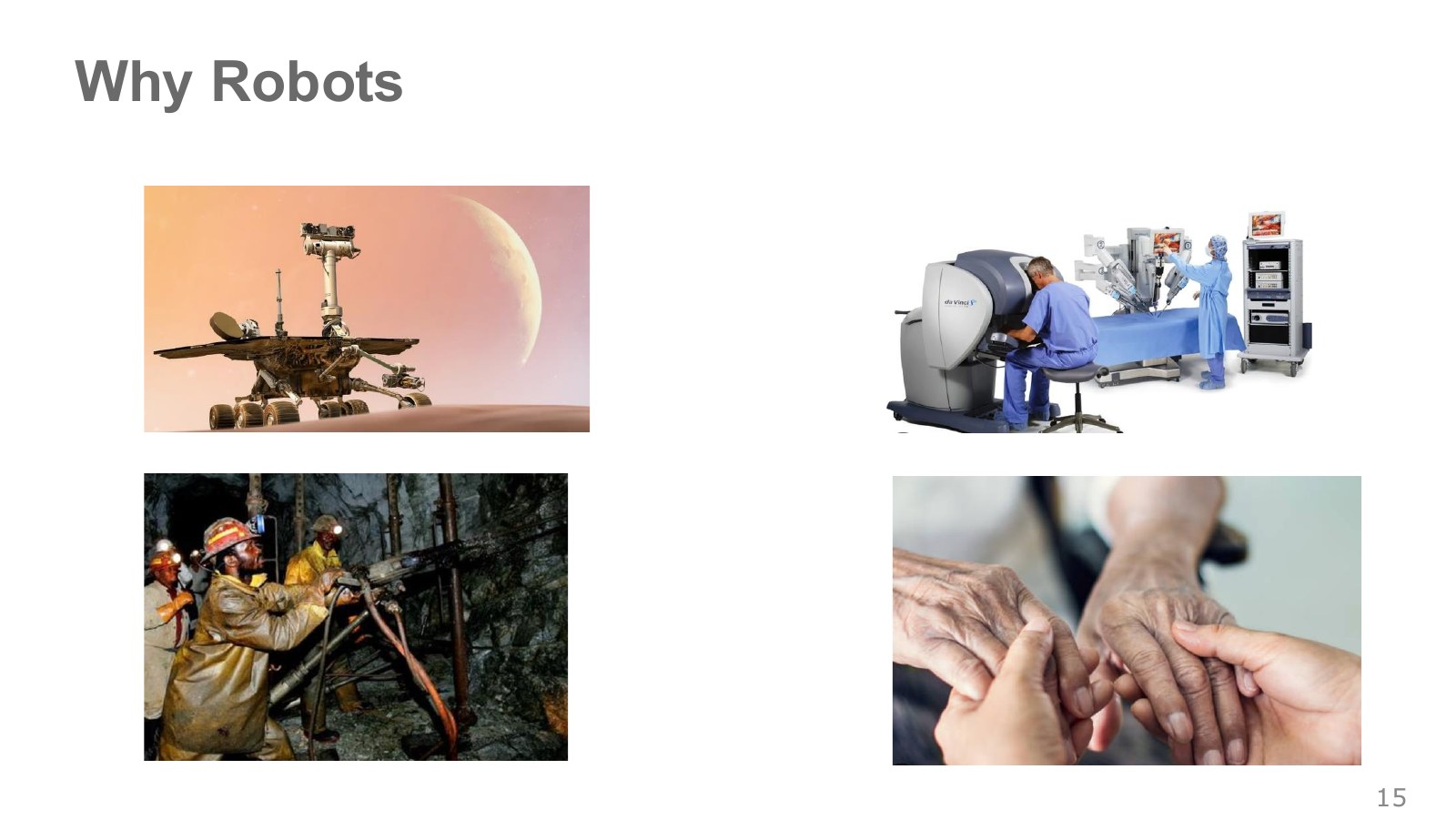
Robots can take on work that is dangerous, distant or repeatedly burdensome for people. Their applications span planetary exploration, disaster response and mining, as well as surgical assistance and everyday care.
These tasks require different capabilities. An exploration robot must make decisions despite communication delays; a surgical system must combine precise movement with human instructions; a household robot must adapt to objects being rearranged every day. Robot learning aims to acquire, from data and experience, the ability to act under such changes.
#P017 · Shakey — sensing, planning and moving
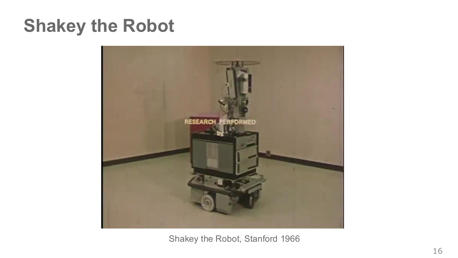
Shakey was an early mobile robot that used cameras and sensors to understand its surroundings and plan routes and sequences for moving objects. It went beyond replaying predetermined motions: it chose a sequence of actions based on the environment it observed.
In the archival video, a television camera observes the scene, range sensors measure distances to walls, and contact sensors detect when the body touches something. A bar at the front can push objects, while planning is computed on an external computer connected by radio. Route finding and planning how to push objects belong to different layers. SRI’s Shakey archive
SRI’s historical account describes Shakey as an SRI AI research project from 1966–1972. “Stanford” on the slide should be read in the context of the institution’s name at the time: Stanford Research Institute. Equating it directly with a present-day Stanford University lab would confuse that institutional history.
The basic flow illustrated here is Sense–Plan–Act: read the environment through sensors, plan actions toward a goal, then drive the actuators.
The lecture also introduces A* through Shakey. A* searches among candidate routes to a goal. We can think of it as adding the cost incurred so far to an estimate of the remaining distance, then choosing the next candidate to examine. Finding a path across a room and deciding the order in which to push boxes with a bar involve different computations. Shakey illustrates a system that turns a perceived scene into symbols and geometry, plans over them, and then moves its body.
The sensors in the video also serve different purposes. A camera may see objects, but contact sensors detect collisions along the body, while the front bar transmits force to objects. When comparing the slow planning discussed in the lecture with today’s control cycles, distinguish the time an external computer spends planning from the time spent driving motors. Even much faster modern systems face the problem that the environment can change while a new observation is being processed.
#P018 · Robotics in structured environments
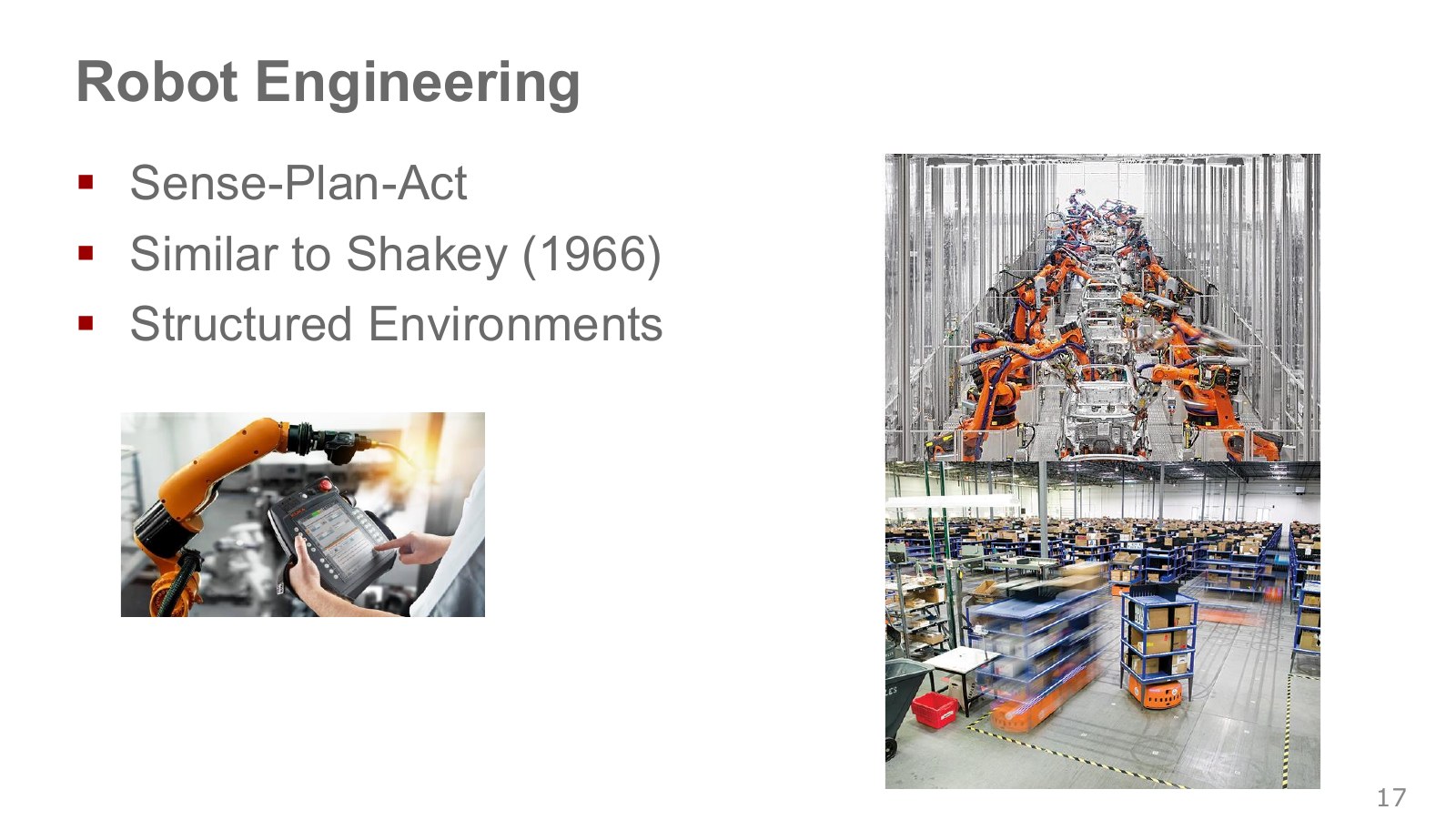
On car assembly lines and in orderly logistics settings, object positions and task sequences can be specified in advance. Robots sense the current situation, plan paths within a known environment and work with high repeatability. This structure has brought major successes in industrial automation.
Unexpected changes expose the difficulty. A part shifts, a person moves an object, or a gripper slips, and the planned sequence may offer no way to recover. The robot needs to adjust its next action to what it observes now.
For a small example, suppose the current position is 0.2 m and the target is 1.0 m. A fixed feedback rule may request , but if the environment limits speed to 0.5 m/s, the position after 0.1 seconds becomes . The next action is calculated from that new position. The loop itself is feedback control; improving its rule through experience is a separate learning step.
I have published an executable Python file, 13 tests, and CSV and result files. This example computes one-dimensional position transitions. The MuJoCo and Isaac Lab examples later in the chapter provide the connection to robot-arm physics simulation.
Unrolled in time, this loop becomes observation₀ → action₀ → observation₁ → action₁. NTU’s introductory lecture, 22:59–23:40 uses the same connection. An action is both an output and a cause of the next input. Predicting actions accurately from stored video and continuing to work in an environment changed by those actions therefore need separate evaluation. Even in the position example, repeatedly sending a speed chosen just once and repeatedly reading the current position produce different trajectories over time.
#P019 · Good hardware can still fail when state estimation is wrong
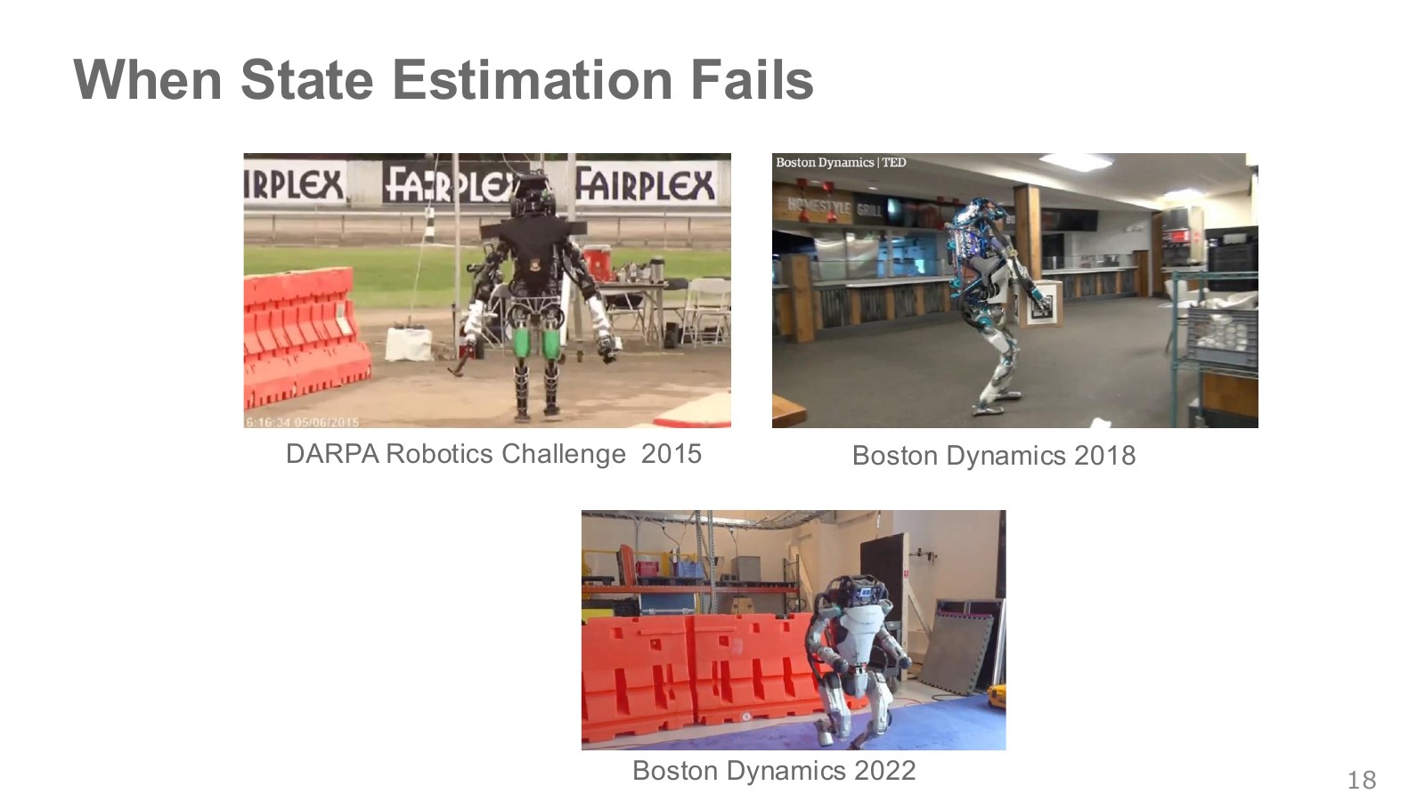
To act, a robot needs to know where its body and nearby objects are. Computing that information from sensors is state estimation. An incorrect estimate of floor height, body tilt or a door handle’s position can make the planned movement disagree with the contact that actually occurs.
Through footage of the 2015 DARPA Robotics Challenge and later Boston Dynamics robots, the lecture shows how sophisticated hardware can remain sensitive to small errors in perception, estimation and planning. If a foot hits an obstacle sooner than expected, for example, the support configuration changes and subsequent movements change with it.
Robot learning offers ways to address these discrepancies through data. Learned policies are still affected by sensor types, delays and the range of errors seen during training, so perception and control need to be evaluated together.
Apply the same questions to the lecture’s door-opening, valve-turning and parkour footage. A handle-position error of a few centimeters can make a hand close on empty space; a different foot placement changes the moment of contact. The square markings visible in the footage are generally visual markers that provide cues for estimating position and orientation. Their presence alone does not establish perfect state knowledge or mean that every movement is performed without vision. The lecture’s point is that mechanical sophistication and reliable environment estimation are separate challenges.
#P020 · Moravec's paradox — an easy movement can be a hard computation
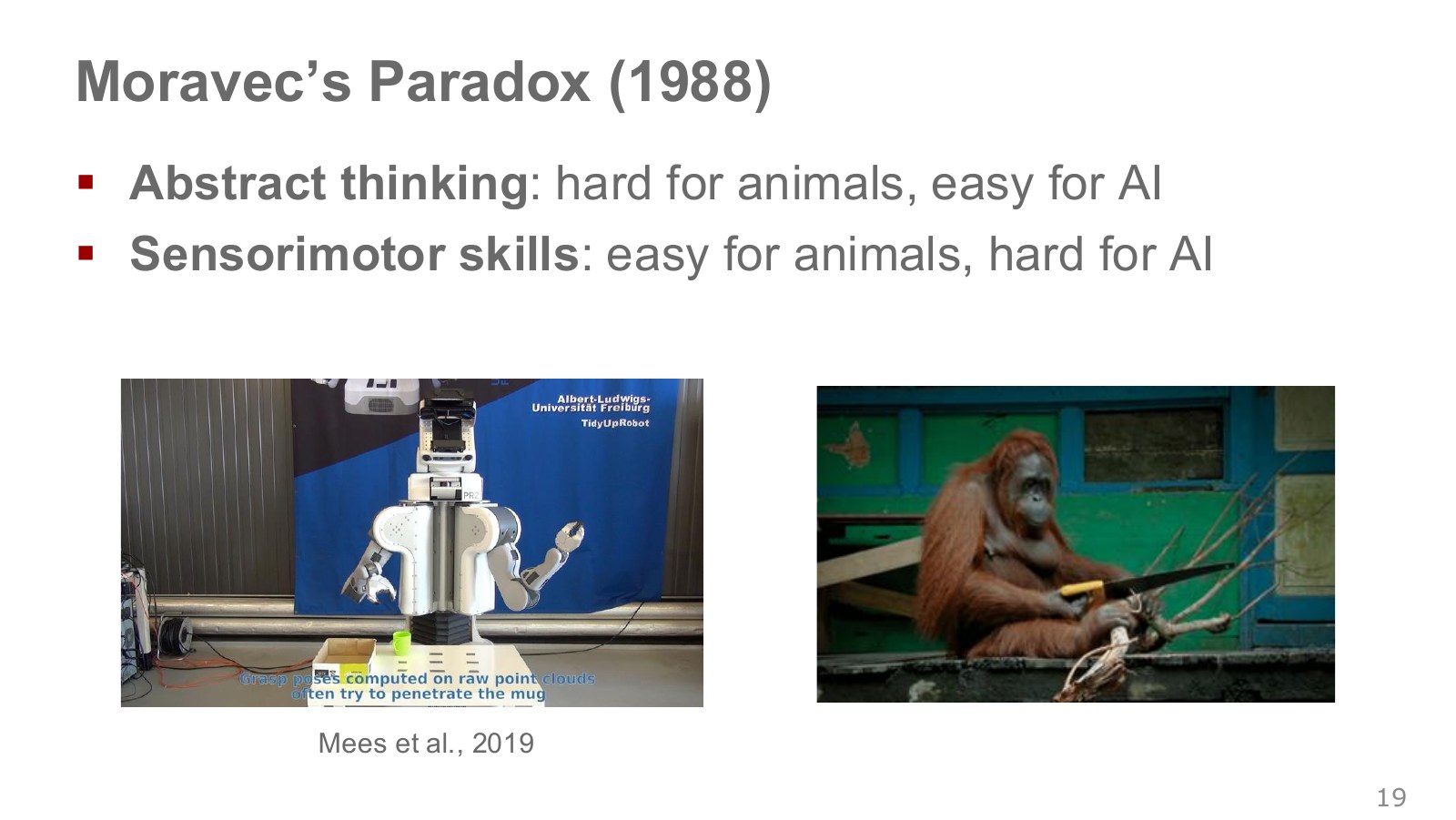
Computers may solve abstract problems that people find difficult while struggling to reproduce the sensory and motor skills that people and animals use naturally. Moravec’s paradox offers a way to understand this difference.
In the PR2 experiment shown by Mees, the robot used a point cloud to estimate a mug’s shape and position and geometrically calculate a grasp pose. During the demonstration, excessive force broke the cup. Choosing where to place the fingertips and deciding how much force to apply after contact are separate problems.
Picking up a cup brings together its three-dimensional shape, material, friction, contact locations and force control. The PR2 example on the left shows the difficulty when an estimated grasp does not fit the cup or the force is inappropriate. The tool-using animals on the right invite us to consider how much experience lies behind ordinary physical skills.
Simply describing a robot’s failure as a lack of intelligence makes it hard to identify what to fix. We need to distinguish a poor object representation, an unpredicted contact and an inappropriate force before deciding what data to collect or which model to change.
#P021 · Where physical robotics meets learning from data
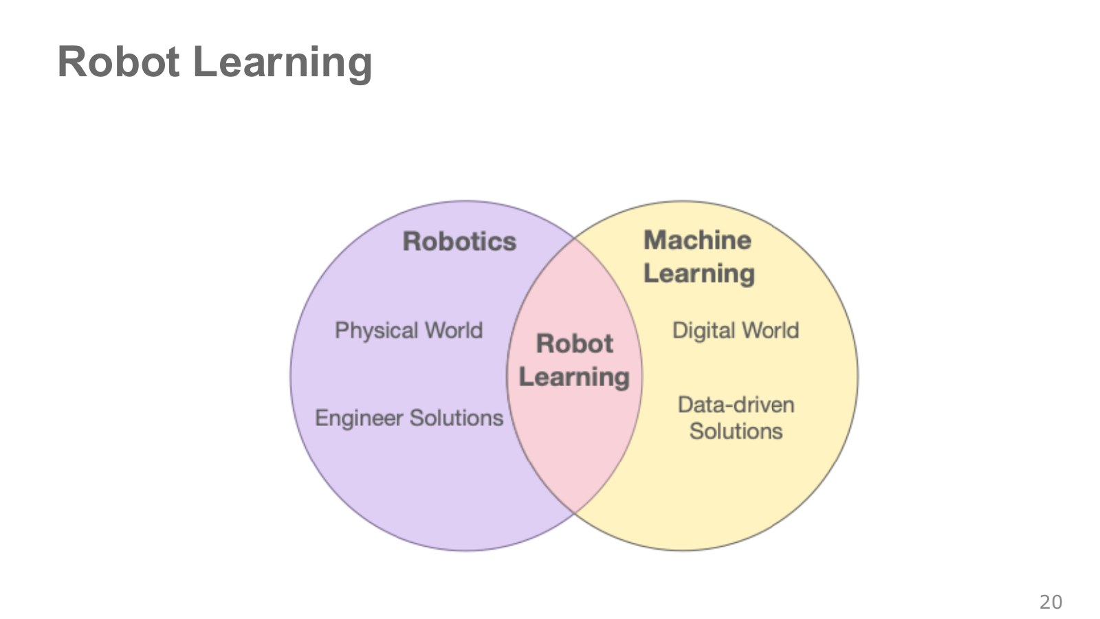
Robotics solves physical-world problems using sensors, mechanisms, actuators and the laws of physics. Machine learning finds recurring structure in data to learn functions that can also handle new inputs. Robot learning lies at their intersection.
Instead of having a person enter the cup’s coordinates every time, a robot can locate it in an image. Instead of hand-writing grasping rules for every object, it can learn actions from diverse demonstrations. Geometry and control still have a place: a system may combine learned perception, calibrated coordinate transforms and a designed controller.
What to learn from data and what to specify through structure and physical models depends on the problem.
#P022 · Separating the problem to solve from the way to learn
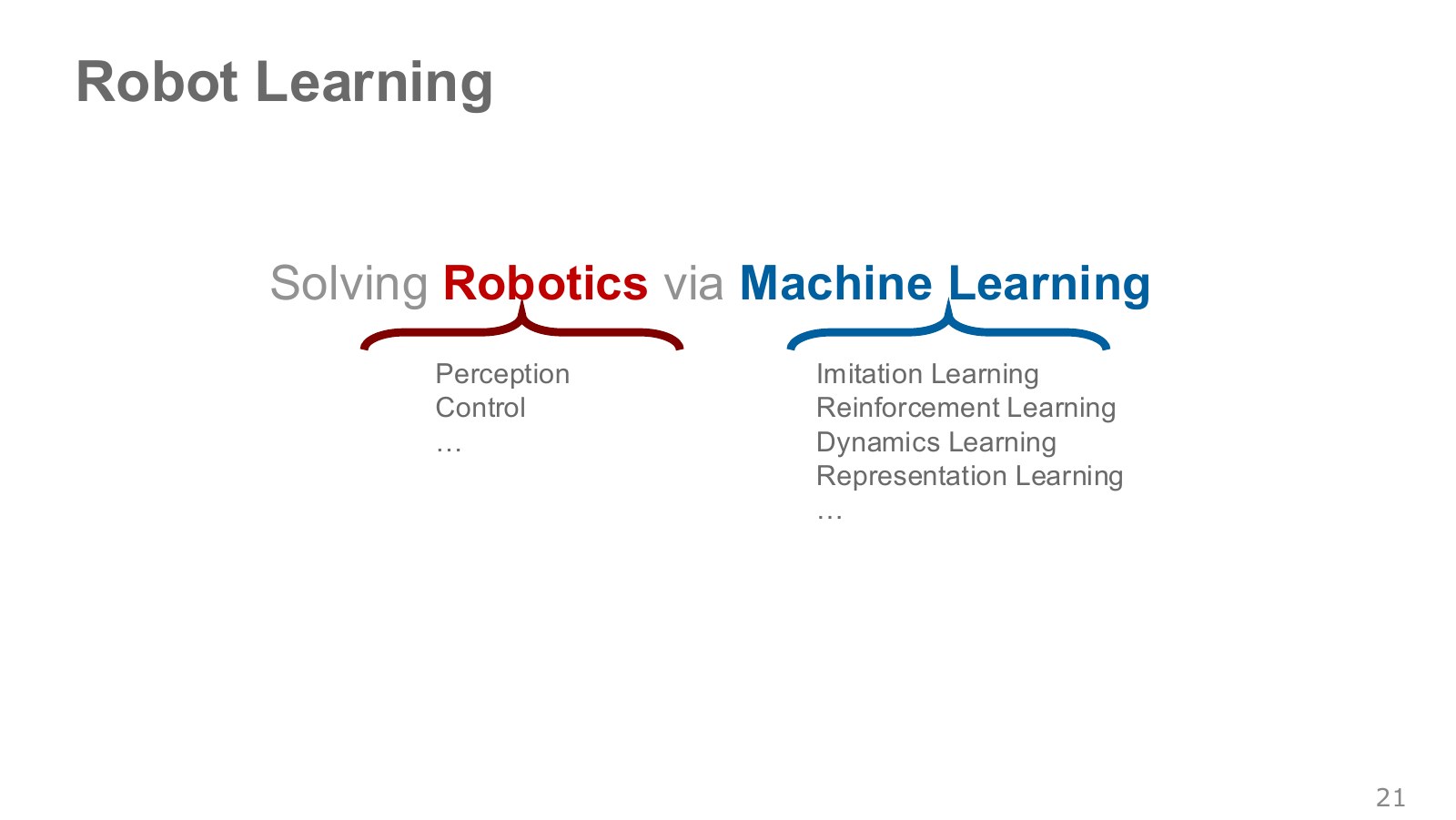
The left side of the slide lists robotics problems, while the right side lists learning tools. Perception concerns how to read the world; control concerns how to move a body.
The learning tools include imitation learning from expert behavior, reinforcement learning from rewards, dynamics learning to predict the state after an action, and representation learning to compress the information that matters.
The same robot arm might use representation learning for camera features, learn an initial policy from demonstrations, and later improve it through task-success rewards. “What kind of robot is it?” and “How was it trained?” are separate questions.
#P023 · How do a dishwasher, a surgical robot and ChatGPT differ?
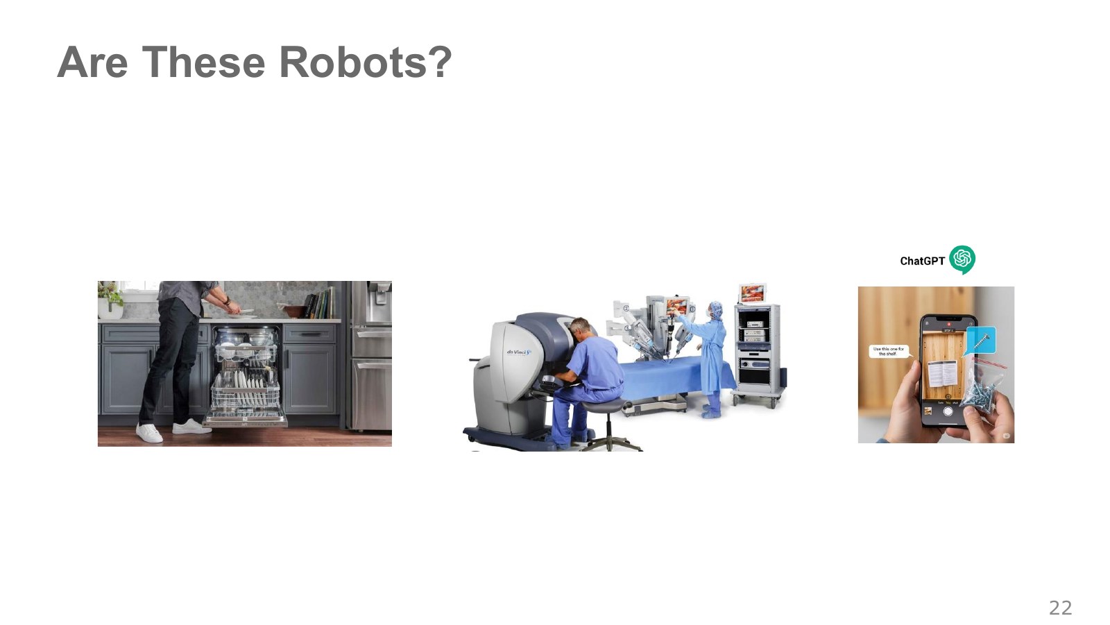
A dishwasher changes the physical world by spraying water and moving mechanisms. A surgical robot translates human input into precise instrument movements. ChatGPT on a smartphone processes language and images, but the application itself has no body that moves nearby objects.
Separate the physical body, who chooses the actions, and what is performed automatically. A teleoperated robot is still a robot, but its control structure differs from that of an autonomous robot. Treating “robotic” and “autonomous” as synonyms loses that distinction.
Robot learning aims to combine physical action with judgment suited to the situation. Reasoning needs to lead to real actions, and the consequences of those actions need to be observed again.
In the discussion at 38:05–40:35 of the ETH video, the useful question is which capabilities to combine, rather than which label to put on each of the three machines. The lecture looks toward combining the reliability of household appliances, the precise physical manipulation of surgical arms and the broad semantic understanding of foundation models. Understanding “put the cup away,” for instance, does not automatically provide repeatable motions or the force control needed to avoid breaking it. A successful system needs those capabilities to connect.
#P024 · Making teleoperated tasks autonomous
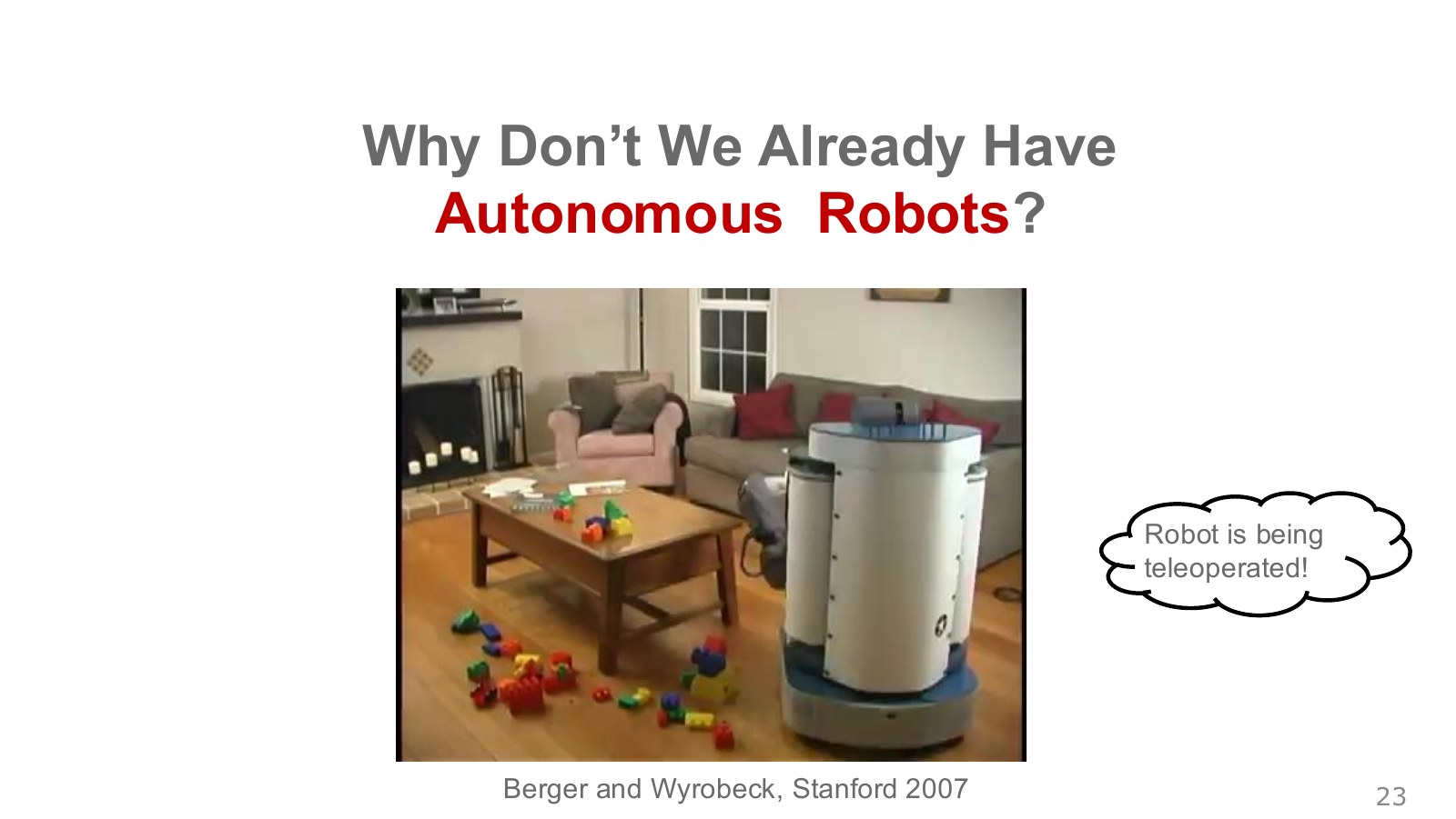
Stanford’s 2007 PR1 video shows a robot tidying objects in a room. The speech bubble on the slide explicitly states that a person was teleoperating it.
The example separates movements the hardware can perform from actions the robot can choose for itself. An arm and gripper capable of moving objects still need a policy to decide which object to grasp, where and how to grasp it, and what to do next.
Teleoperation is also used to collect training data. The observation–action relationships demonstrated by a person can be recorded and used to train a policy. A successful human-operated demonstration and the autonomous execution of a learned policy nevertheless need to be distinguished.
Saving successful videos alone is not enough to create demonstration data. The camera and joint observations that the policy will receive at execution time need to be synchronized with the actions the person took at those moments. NTU’s imitation learning lecture, 5:14–7:49 explains how expert interaction records become an observation–action learning problem. Whether a person physically guides the arm or teleoperates it, the result must be trainable pairs: given this information, which command did the person issue?
#P025 · Robot hardware and GPUs have advanced together
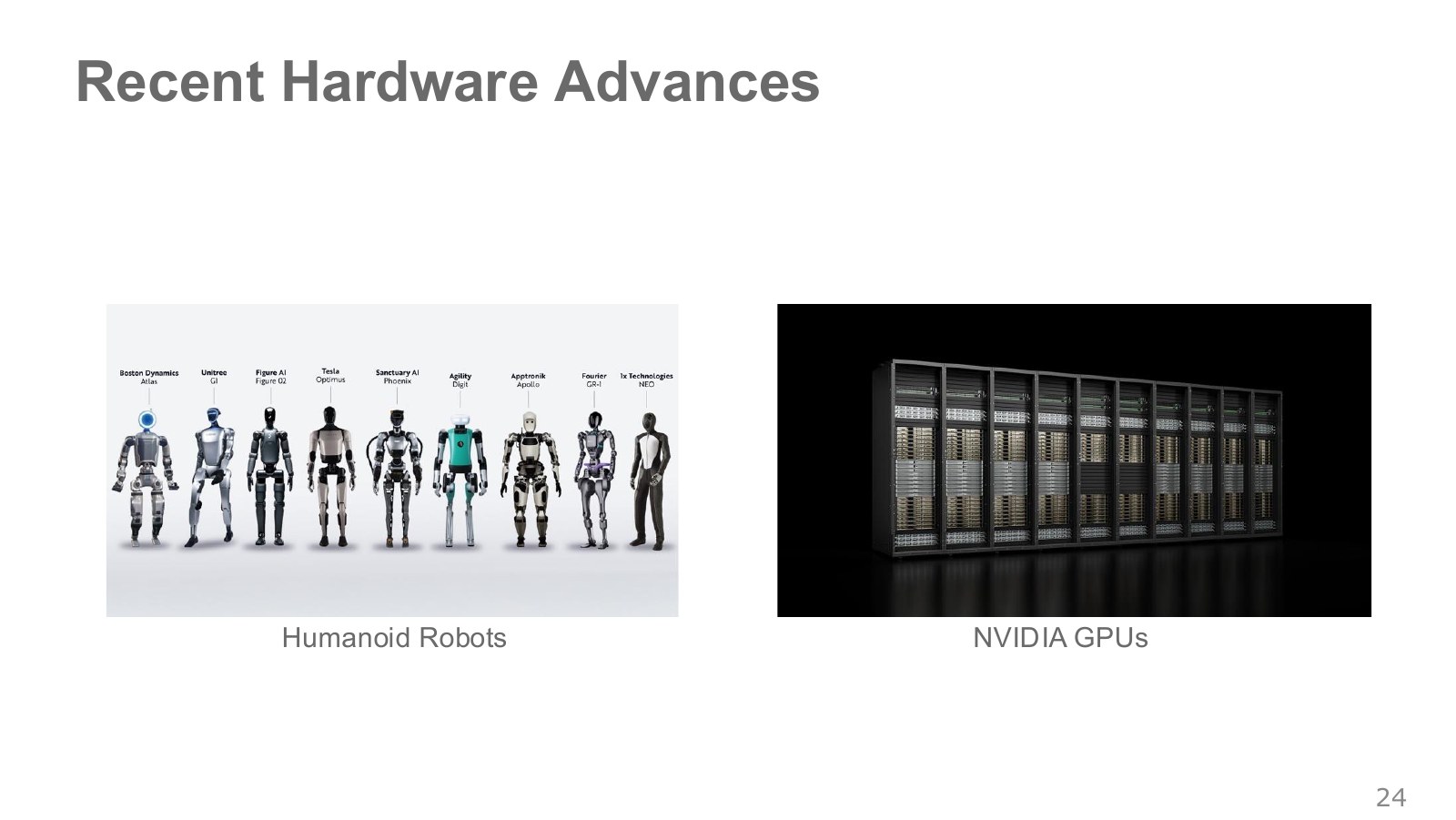
The slide places a range of humanoid platforms on the left and NVIDIA GPU systems for large-scale training on the right. As robots have gained a wider range of movements, computational resources have also grown to support larger models and more data.
The two advances address different bottlenecks. Hand mechanisms and actuators determine possible contacts and forces; computational resources affect the scale of training and inference. A capable body alone does not produce intelligent behavior, and a large model still needs an action interface.
For a small exercise, first establish what observations, actions and rewards mean. Then use parallel simulation or GPU training where it addresses an actual bottleneck.
#P026 · The scale of data behind AI's progress
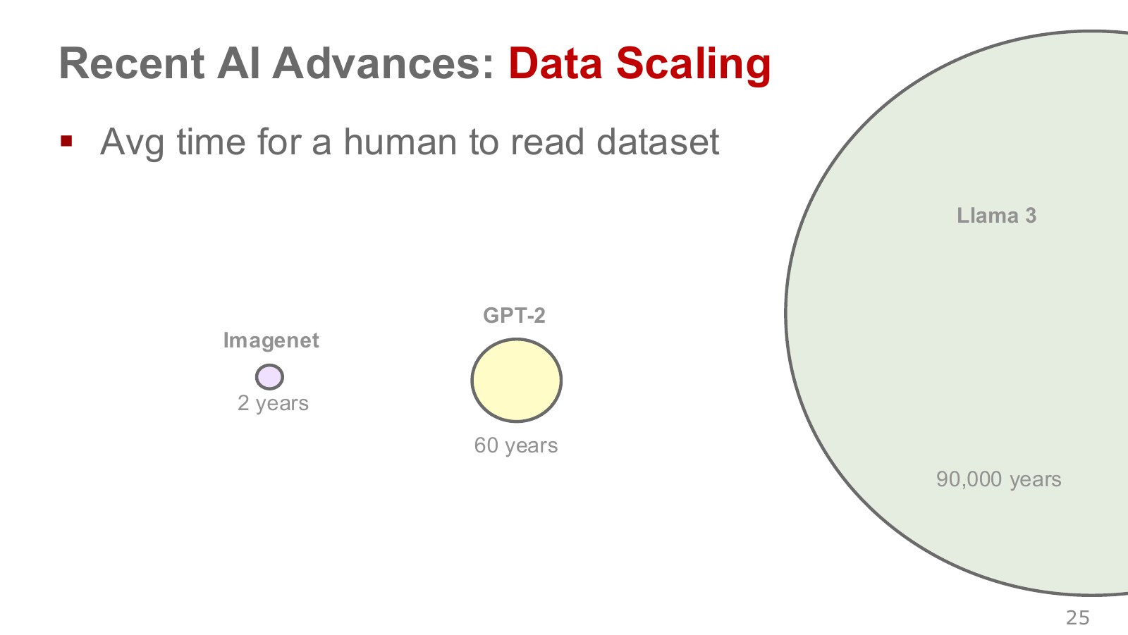
The lecture compares ImageNet, GPT-2 and Llama 3 by estimating how long it would take a person to read or view their data. The point of the analogy is that recent models learn from more information than one person could readily experience or read.
The “time for one person to read the data” is an analogy to make scale tangible. Viewing an image and reading text use different speed assumptions, so neither the areas of the circles nor the ratios of years can be read as ratios of training cost.
The years on the slide are illustrative conversions used in the lecture. The circle sizes do not represent precise proportions either. Image counts, text-token counts and robot-trajectory counts use different units; placing their numbers side by side cannot by itself compare learning difficulty.
For robot data, diversity of tasks, objects, environments and robot bodies matters alongside quantity. Many consecutive frames of the same scene and trajectories covering different failures and recoveries provide different information.
Counting consecutive frames as independent experiences can exaggerate diversity. DeepMind/UCL Lecture 1, 1:15:41–1:16:11 explains that a robot moving within one room receives strongly correlated inputs over time. Thousands of views of the same cup from slightly different angles and dozens of attempts to recover an occluded, slippery or dropped cup supply different kinds of experience. Alongside trajectory counts, examine the variation in environments, objects and initial conditions.
The numerical conversions help convey the analogy’s scale. Assuming one person reads or views the data, the lecturer gives roughly two years for ImageNet, 60 years for the GPT-2 corpus and 90,000 years for Llama 3’s training data. These illustrative conversions depend on the processing-speed assumptions used in the lecture. They do not imply that a robot must be teleoperated for those lengths of time. Use them to think about the cost difference between collecting images and text from the internet and collecting physical actions together with their consequences.
#P027 · Models have expanded from perception to strategy and multimodal understanding
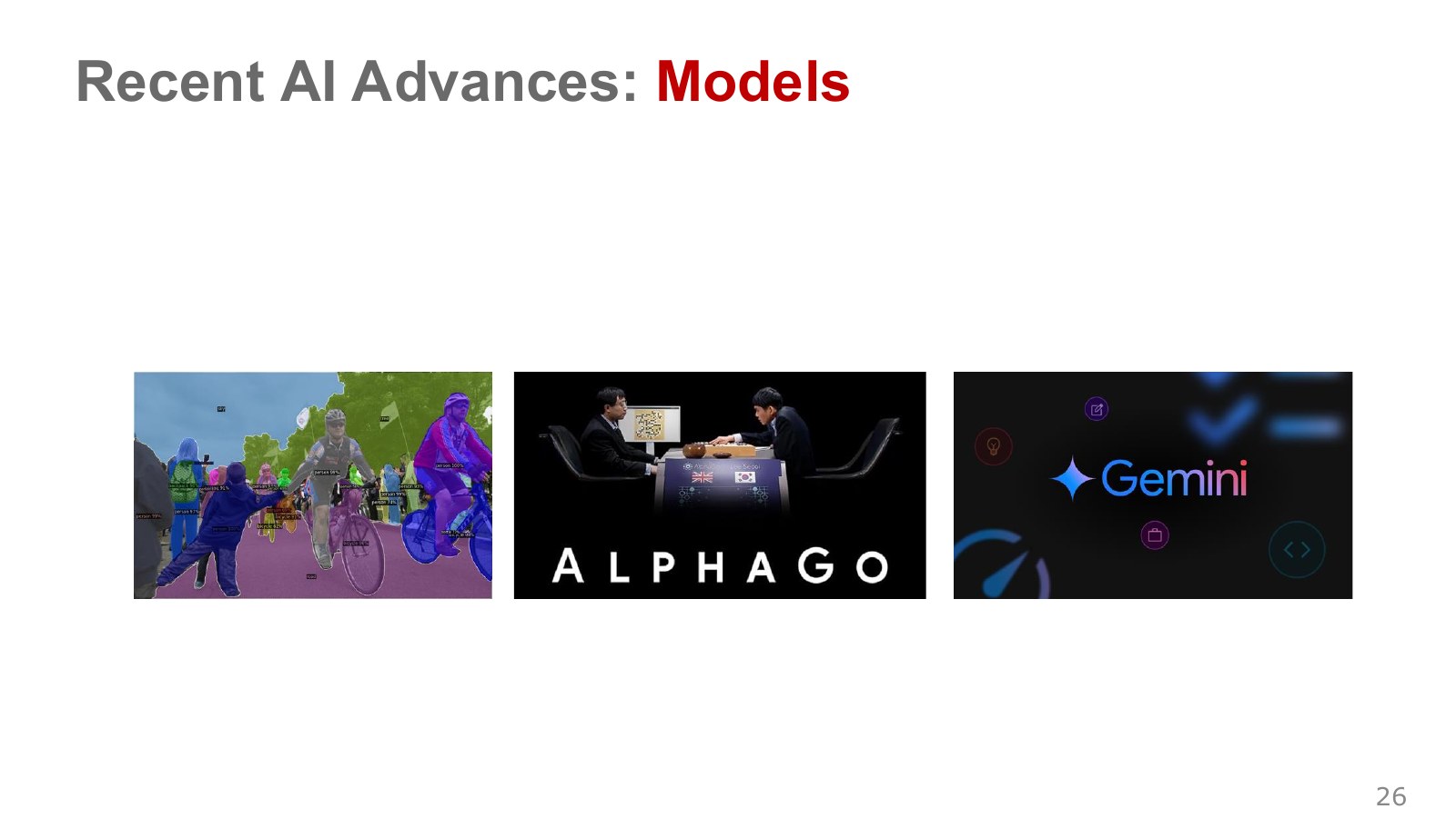
A model that identifies objects pixel by pixel, AlphaGo choosing moves with long-term consequences, and multimodal models handling several input types demonstrate different AI capabilities.
Robots connect these capabilities. They may need perception to find a cup, judgment to choose a task sequence and an understanding of a spoken goal. These abilities need not be trained with the same learning signal.
Ground-truth segmentation masks, demonstrated actions and win/loss rewards in games define different objectives. Bringing an advance into robotics requires examining the training data, objective and execution conditions alongside the architecture.
The lecture highlights AlphaGo’s move 37 in its second game against Lee Sedol as more interesting than the victory itself. The move initially looked unfamiliar, but its value emerged later in the game. For robot learning, the question is whether a system can go beyond reproducing movements specified by people and discover a new sequence that works within a goal and environmental constraints. Go has explicit rules and a clearly computable win/loss outcome. Transferring such discovery to robots with uncertain physical contact leaves further questions about rewards, exploration and evaluation. DeepMind’s account of the game
#P028 · Generalist robot policies beyond a single task
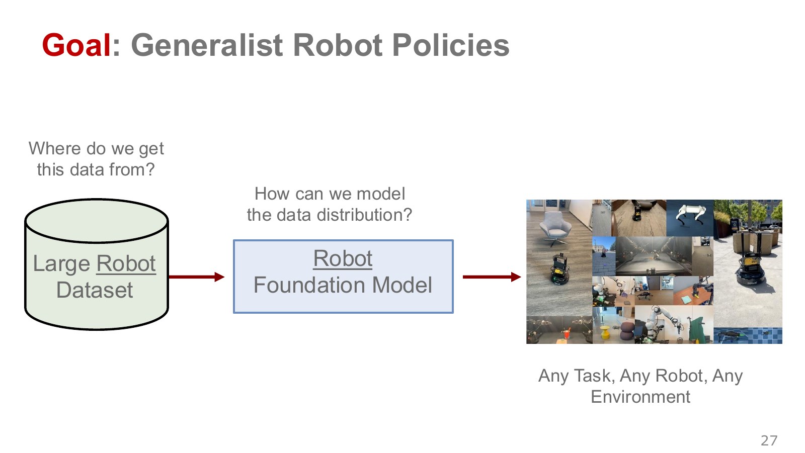
A generalist robot policy aims to move beyond picking up one object at one location toward policies usable across multiple objects, tasks and robots.
The figure links large robot datasets to models that produce a range of robot actions. This goal raises two questions: where can we collect diverse experience, and what kind of model can represent its heterogeneous distributions?
“Generalist” becomes clearer when we separate the axes of evaluation. Adapting to a new cup, moving through a new room, following an unfamiliar instruction and transferring to a robot with a different joint structure are different generalization problems.
The generalist-policy discussion in ETH Lecture 1, 47:20–48:10 considers both data collection and modeling heterogeneous distributions. Turn that into an evaluation question: which combinations appeared in training, and which were first encountered in the test? Training on a red cup and a blue bowl and testing on a blue cup measures a different capability from transferring to an unfamiliar gripper. Success on several tasks alone does not establish immediate applicability to every robot.
Page 2 of the RT-2 paper distinguishes using web-learned semantic understanding to recombine existing robot skills from acquiring entirely new physical skills. A robot that has learned to pick and place objects may apply that skill to a new semantic instruction such as “put it next to that number.” This does not mean it has acquired every form of tool use or complex contact behavior absent from its training data. When assessing generality, ask separately whether the robot understands the reference and whether it can physically perform the required motion.
#P029 · The ambition of downloading a robot's brain
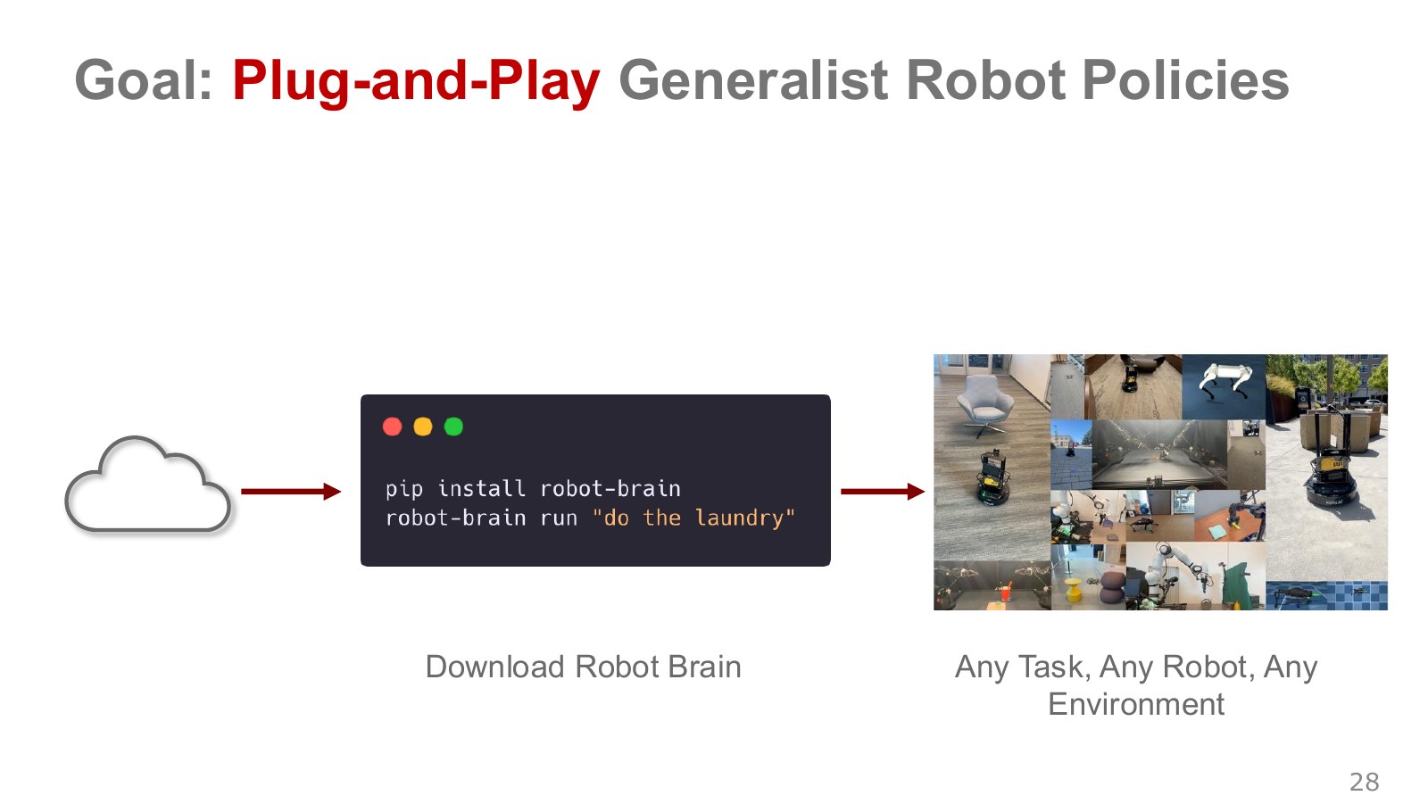
What if we could obtain a trained policy and connect it to a robot as easily as installing a software package? The robot-brain command on the slide illustrates that ambition. It should not be read as an installation guide for an actual package.
Reaching that goal requires agreements beyond a model file. Camera-input ordering, the meaning of joint states, action units, coordinate frames, normalization and command timing all need to be compatible.
An output of 0.1 has different consequences if it means a 0.1 m displacement, a 0.1 m/s velocity or a normalized joint target. Matching model inputs and outputs to the robot’s real sensors and actuators is central to deployment.
#P030 · Shared datasets and robot foundation models
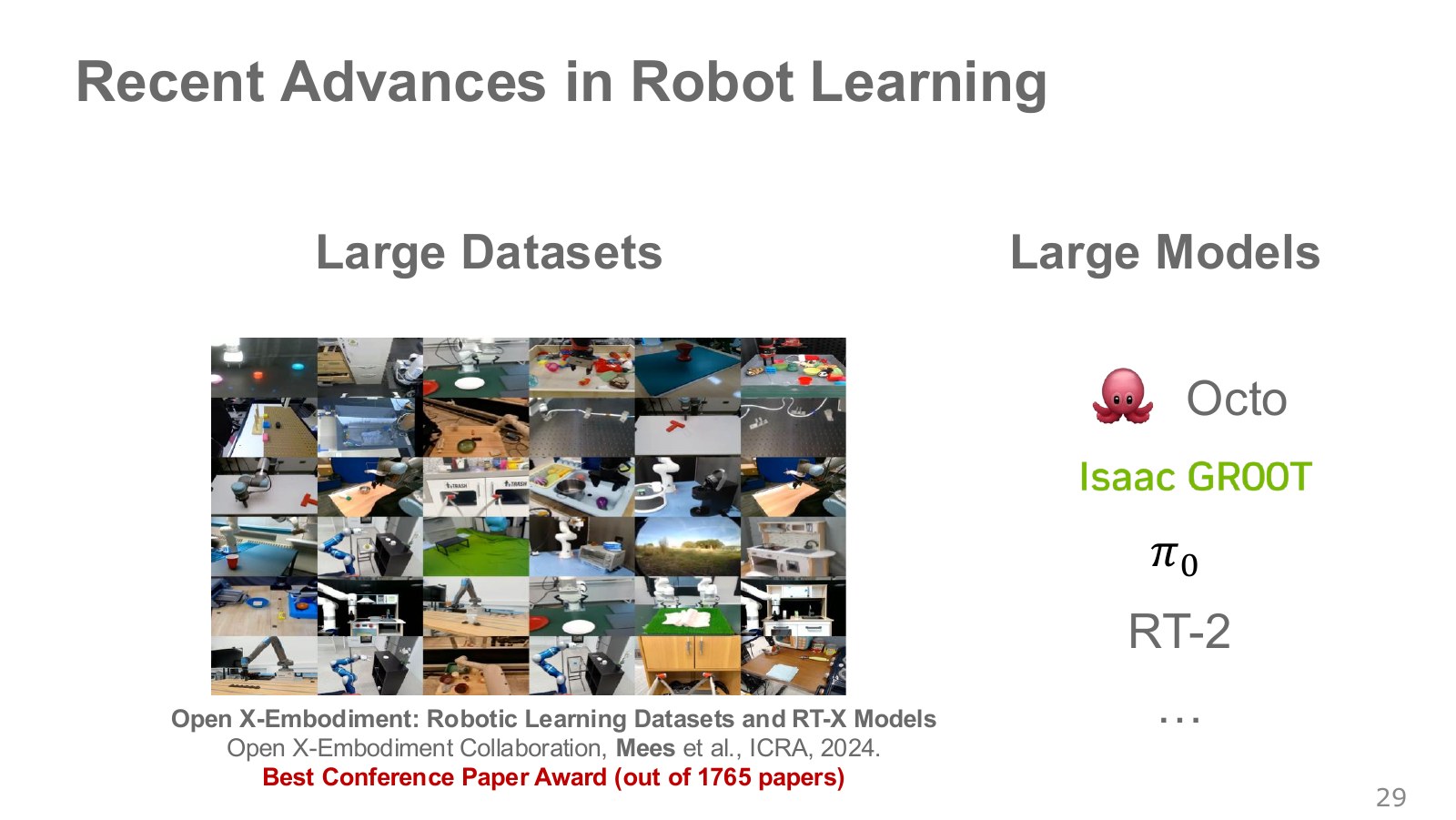
Open X-Embodiment is a prominent example of research using data from multiple robots. Bringing observations and actions into a common format creates a basis for applying one platform’s experience to other tasks and robots.
The right side of the slide includes Octo, Isaac GR00T, and RT-2. Their differences become clearer when we compare the data they use and the actions they output, rather than treating them as one algorithm.
When reading the public data and code, start with action dimensions and units, camera arrangements and the criteria for starting and ending a trajectory. Combining datasets does not automatically align what their entries mean.
The original project’s stated scale is over one million real trajectories across 22 robot embodiments, with the initial collaboration bringing together data from 21 institutions. Combining existing records from multiple labs in a common format made that scale possible. Do not equate a large participant count mentioned in a transcript directly with the number of institutions: distinguish embodiments, labs, institutions and individual researchers. To understand the diversity available to a generalist model, examine both the number of files and the bodies and actions they contain. Original Open X-Embodiment project
#P031 · A policy maps observations and instructions to actions
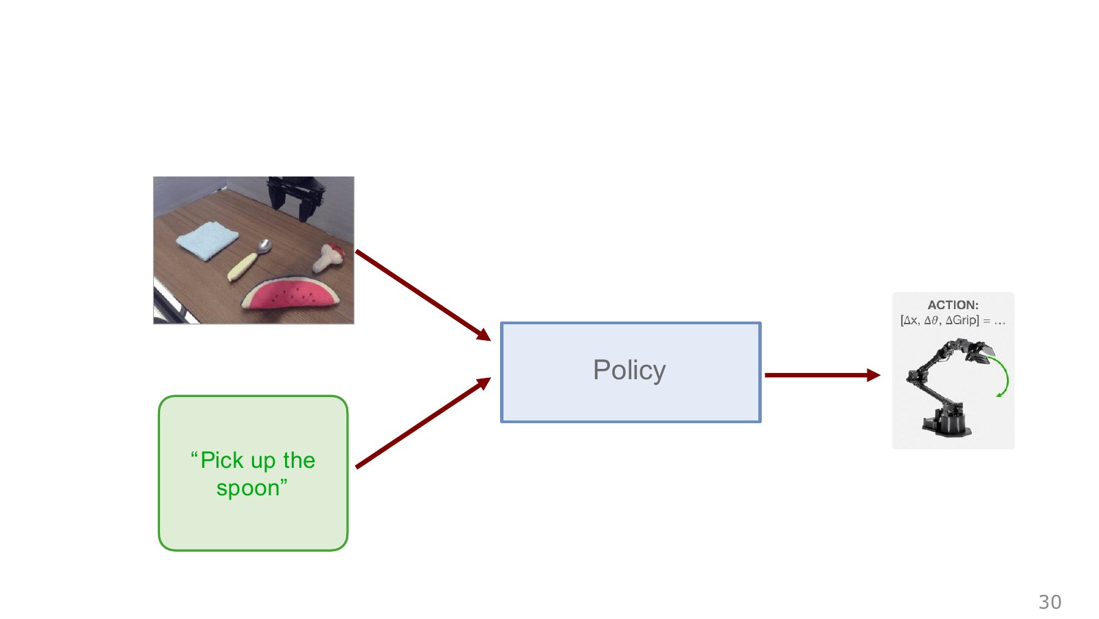
Suppose a robot sees a spoon among other objects and receives the instruction “pick up the spoon.” The policy reads the current image together with the instruction and decides how to translate and rotate the hand and when to close the gripper.
The action notation on the slide includes changes in position and orientation, plus the gripper state. Some models predict actions for several time steps at once, but the basic connection remains observation and goal → policy → action.
An observation is the information available to the robot. Occlusion and sensor error can keep it from containing the full physical state. That motivates using earlier observations or estimating an internal state.
DeepMind/UCL Lecture 1, 43:52–45:17 uses a camera-equipped robot facing a wall. If the current image shows only the wall, it cannot reveal what lies behind the robot or where it has just come from. The appropriate next action can depend on the route taken, even when the current image is identical. This is partial observability: one current observation may not contain enough information to predict the consequences of actions.
In our spoon example, when the hand obscures the spoon, the current image alone may not establish whether the grasp succeeded. Earlier images, the gripper’s opening and force sensors can supply additional information. The agent’s internal state is a representation for carrying available information forward to the next step. We should distinguish the full physical state, one camera image and the model’s internal memory when using the word “state.”

In the maze at 47:31–51:08 of the UCL video, the robot sees only a few nearby cells. The two highlighted regions occupy different positions but have the same local pattern. From the upper right, reaching the goal at the upper left requires going down and around; in the left corridor, the robot should go up. A deterministic policy receiving only the current image has no information to distinguish the views, so it produces the same action and cannot choose a shortest-path action in both situations.
We cannot immediately conclude that adding the two most recent images solves the problem either. Two images can still look the same after movement through similar corridors. The robot needs distinguishing information, such as movement history, a position estimate or another sensor. Extending memory and actually obtaining the information required by the task are different things.
#P032 · Using the same input structure to describe a scene
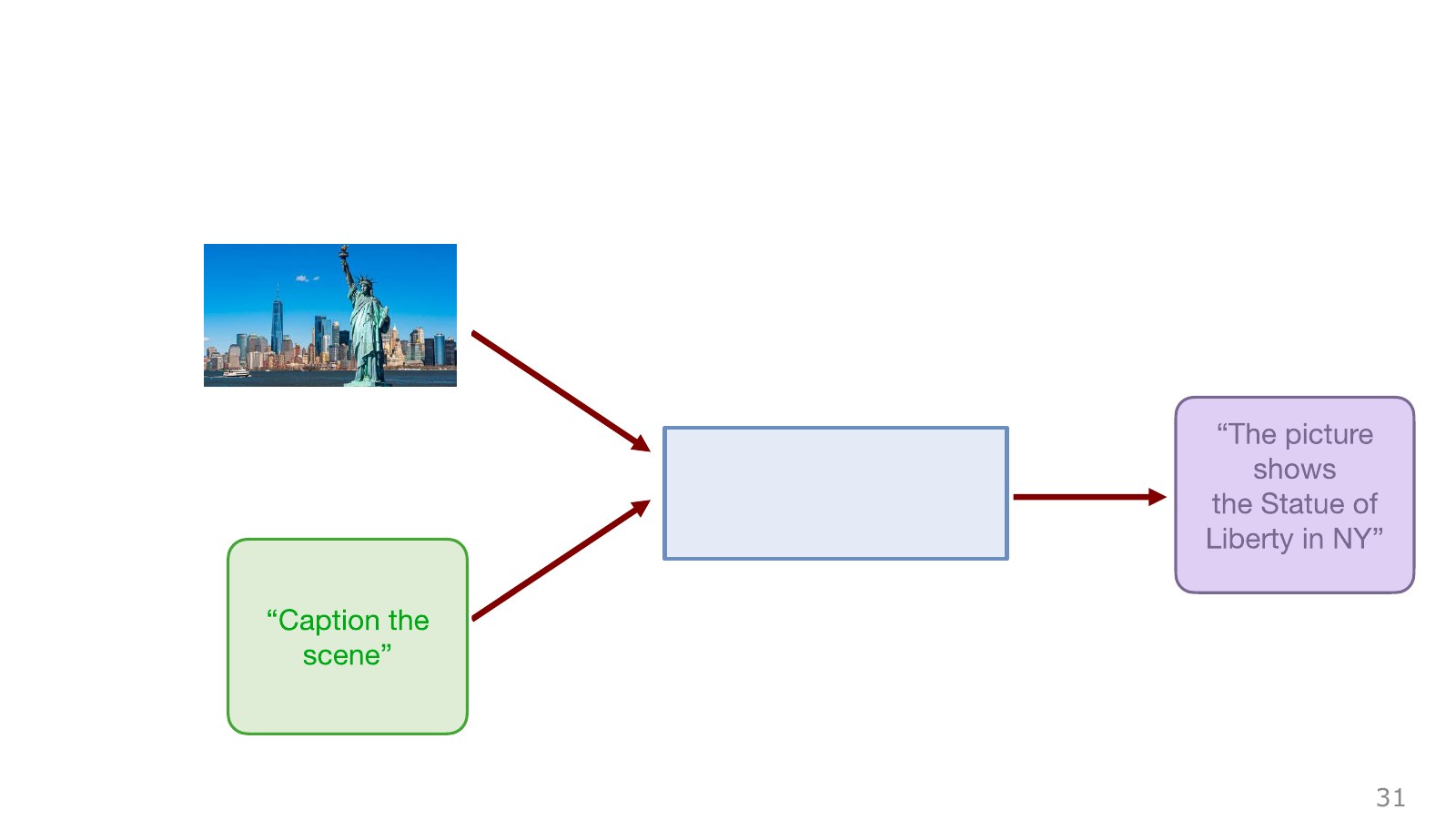
Now replace the scene in front of the robot with a photograph of the Statue of Liberty and ask for a description. The input still consists of an image and a language instruction, but the output is a sentence rather than an action.
This comparison suggests a way to connect robot policies with existing vision-language models. We can build on their ability to extract meaningful image features and relate them to instructions, then train the final output to produce robot actions.
Describing a spoon on a table and physically picking it up are different capabilities. The latter includes consequences involving contact, force and timing.
#P033 · Connecting VLM knowledge to a robot policy
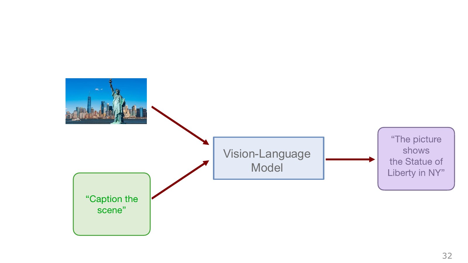
A vision-language model (VLM) handles images and language together. Representations learned through captioning or visual question answering can help connect the meanings of objects with task instructions.
In a robot system, we might send the model’s description to a separate planner or train the model to output actions directly. A model that also outputs actions is called a VLA.
Saying that a system uses a VLM therefore leaves its overall control structure unspecified. To understand the system, trace where information is interpreted, where actions are chosen and where they are converted into real commands.
#P034 · Treating robot actions as multimodal sequences
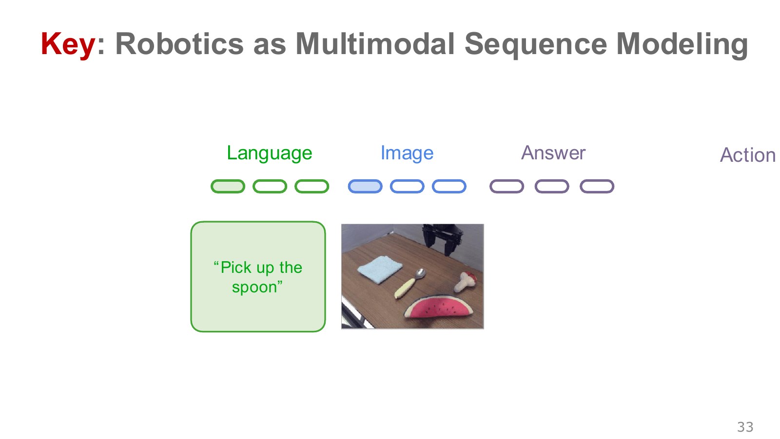
Just as language can be represented as a token sequence, images and actions can be converted into sequences of representations that a model can process. This formulates the connection among images, instructions and actions as multimodal sequence modeling.
For example, the input may combine language tokens for “pick up the spoon” with a representation of the current image, while the output contains values or tokens representing robot actions. RT-2 provides a concrete example of representing actions as text tokens.
Aligning representation formats does not remove an action’s physical meaning. A decoding step and a control interface must interpret the output as position, rotation and gripper commands before a robot can move.
At 50:12–52:20 of ETH Lecture 1, the image–instruction–action structure of a robot policy is compared with the image–question–sentence structure of a scene-description model. Sharing a computational framework for input and output sequences lets us bring learning techniques from vision and language into robotics. But a predicted action changes the world and creates the next observation. Even if the model predicts “close the gripper,” closing too late can miss the spoon, leaving the next step with an input unlike the successful demonstration. This is why we examine action-token accuracy alongside success over the whole task.
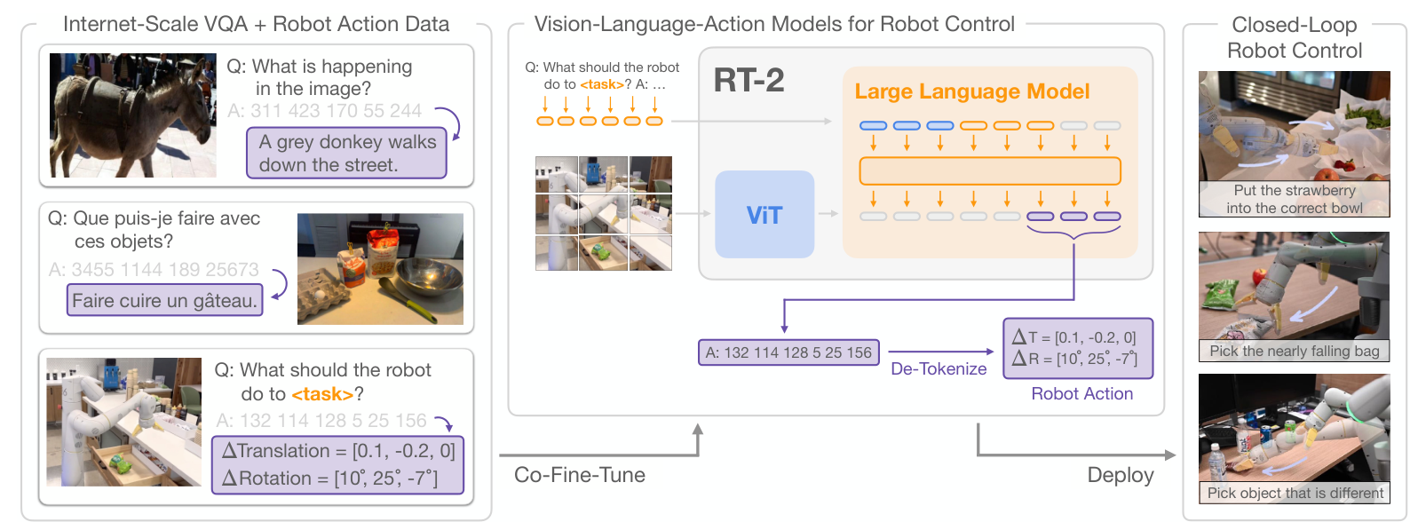
On the left of the original figure are two kinds of training data: vision-language examples that answer photographs with sentences, and examples that answer robot-camera observations and instructions with actions. In the center is the model fine-tuned on those data. ViT is the visual encoder that converts images into representations the model can process. The purple output tokens are decoded back into robot commands such as translation and rotation.
The closed loop on the right keeps receiving observations after actions and feeding them back into the model to compute the next command. It does not generate one command and proceed without looking until the task ends. Decoding tokens into actions still requires the action format used in training and the robot’s interface. Outputting the string “132” alone specifies neither its units nor its physical meaning.
#P035 · Is training a large Transformer enough?
If one model can handle images, language and actions, does the remaining challenge simply become making it larger? Here the lecture turns to what makes robotics different.
Robot data requires collecting real actions, models must respond within time constraints, and evaluation takes place in the physical world. A sentence that finishes a little late has different consequences from a delayed command to a robot maintaining its balance.
Alongside model scale, we must design the training data, determine whether actions can be produced at the required frequency, and decide how to evaluate the system when the environment changes.
#P036 · Scaling data, models and evaluation together
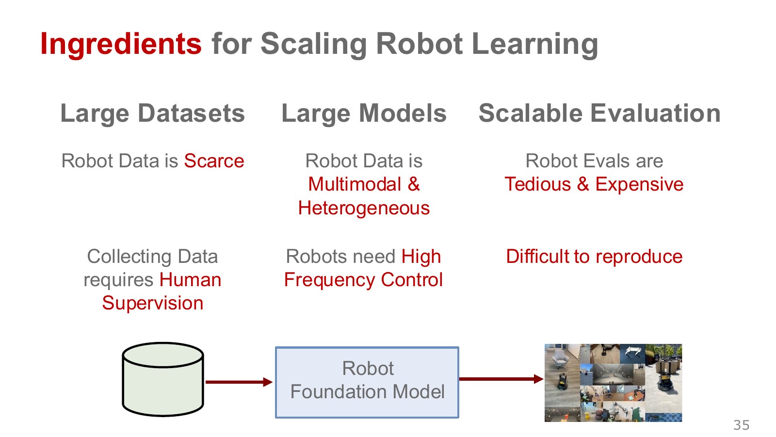
The first challenge is data collection. Human-teleoperated and supervised trajectories are expensive to gather. Video, joint measurements, forces and other sensor signals also need a shared time base.
The second is different robots and real-time execution. Robots have different sensors, actuators, action dimensions and units. For a computationally heavy model, we must also examine inference latency in relation to the control cycle.
The third is evaluation. Real-world experiments cannot easily reproduce identical initial conditions, and resetting objects or recovering from failure costs time and effort. We therefore use simulation, repeated experiments and records of human intervention together to understand performance.
ETH Lecture 1, 52:57–54:36 moves through scarce data, different sensing and actuation, real-time execution and the cost of real-world evaluation. Connecting these issues in an experiment requires a timeline: observation acquired → inference completed → command applied → outcome measured. An environment requesting new commands at 10 Hz allows 100 ms between actions. If inference takes 150 ms, a synchronous system that computes a new action at every step cannot maintain that rate. This execution constraint needs checking independently of semantic understanding. Predicting action chunks or separating slow planning from fast control can address such constraints, but must be validated through actual latency and behavior.
#P037 · Learning signals in imitation and reinforcement learning
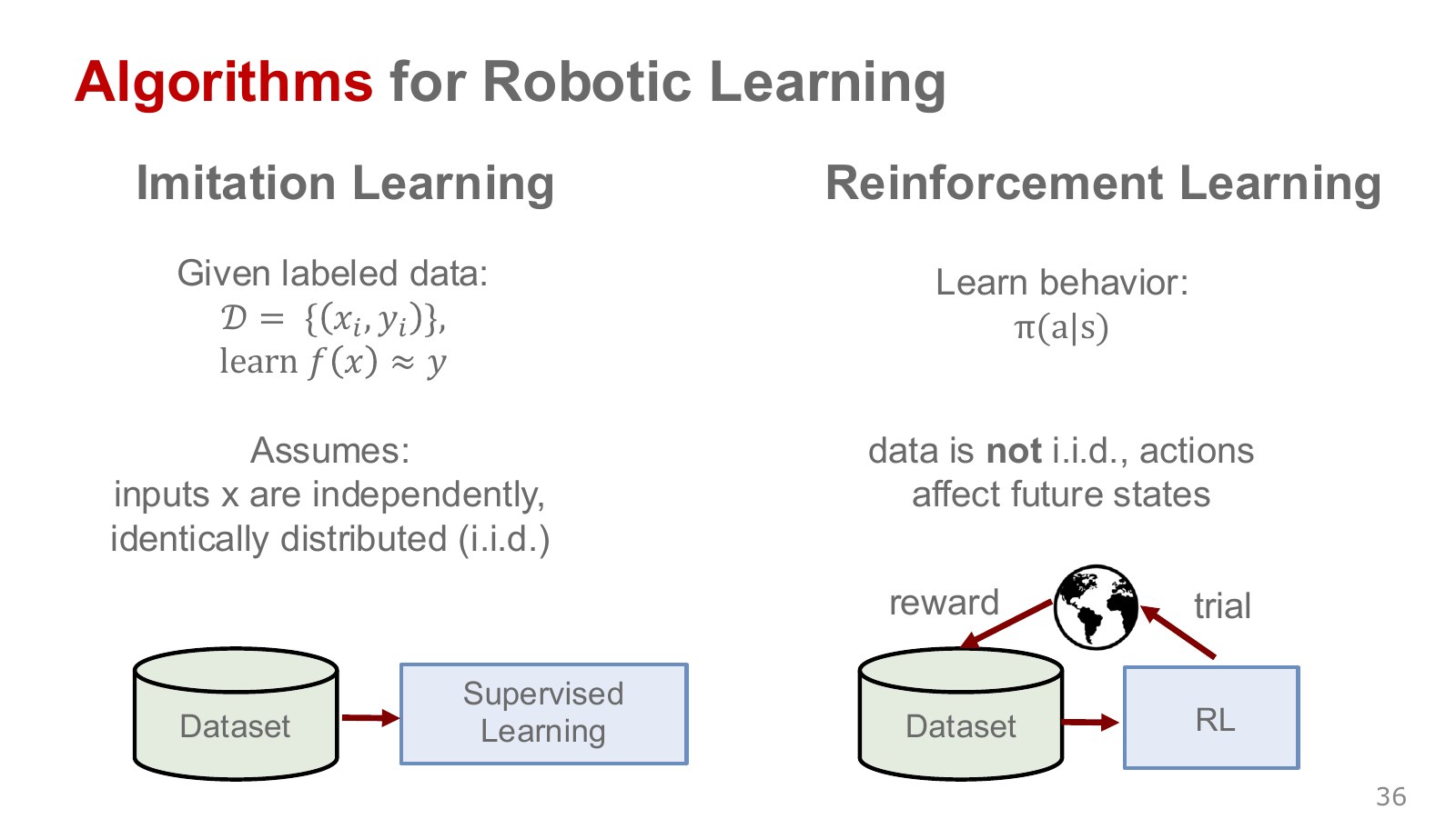
Imitation learning learns which action an expert took under a given observation. A common starting point is behavior cloning: training a prediction function with observations as inputs and demonstrated actions as targets.
Reinforcement learning improves a policy using rewards from the consequences of actions. Because an action changes the next state, learning must consider subsequent outcomes as well as the immediate reward.
IID on the left of the slide refers to the independent and identically distributed assumption used in classical supervised-learning analysis. Real robot demonstrations are temporally connected trajectories, and an imitation policy changes subsequent observations when executed. The slide should not be read as saying imitation data is always independent. The DAgger paper provides a connection to policy-induced observation distributions and accumulating errors.
A policy trained only on demonstrations centered over a cup may encounter unfamiliar images after drifting slightly off-center during execution. Small action errors change the next input: this is a defining feature of sequential decision-making.
A reward differs from a label specifying the correct action at every instant. NTU’s introductory lecture, 2:10–3:47 starts from the idea that the quality of an outcome can be a learning signal even when the best output is difficult to specify directly. Giving a robot +1 for placing a cup on a shelf does not tell it at every moment which way to reach or when to close the gripper. It must connect the sequence of choices leading to success through experience.
A reward is a signal received on one transition; a return accumulates rewards over subsequent steps. In NTU’s game example, 8:29–10:19, moving sideways may score nothing immediately but prepare a successful attack. A robot may first move its hand away from the cup, apparently away from the goal, yet avoid a collision and enable later success. Treating every action without an immediate score as bad would prevent learning such sequences.
The numerical definition of the goal also changes behavior. DeepMind/UCL Lecture 1, 16:31–17:13 describes giving −1 at every step before reaching the goal. Under the stated conditions, arriving in five steps produces −5, while taking 20 produces −20, favoring faster arrival. The objective now includes speed as well as success. This does not mean two reward designs always yield the same optimal behavior; termination conditions and time limits also need to be specified.
Conditions omitted from a reward can make the training objective diverge from real success. NTU’s imitation learning lecture, 3:29–4:36 illustrates this with a plate that reaches its target but breaks along the way. Evaluating position alone leaves damage out of the objective. For moving a cup, we must decide how target position, breakage, spilling and elapsed time enter the success criteria and reward. Imitation learning offers a way to supply examples of the desired behavior through demonstrations, but does not automatically solve situations beyond them.
NTU’s account of behavior cloning, 7:54–9:01 notes that an expert who always drives well may leave no examples of recovering after approaching a wall. In robotics too, collecting more successful demonstrations and teaching recovery from the off-course states a policy actually visits are different data-collection tasks. First identify the missing situations, then add demonstrations or corrections in those states.
Comparing the equation on page 13 of the original NTU PPTX with the PDF gives the simplest form of a return.
Explore the symbols and calculation Total episode reward sums step rewards from 1 to
Read the equation in words
Add all rewards received during one attempt in order. The equation distinguishes a score at one step from the score over the whole task.
Understand each symbol
- The sum of rewards in one episode. This symbol is distinct from a rotation matrix used in other equations.
- The reward received at one step: a learning signal defined so that larger is better.
- The length of a trajectory or sequence. Here it sets how many steps enter the sum or product.
- The index of a step at which the robot acts in the environment, distinct from elapsed time in seconds.
- Add every term over the indicated range, computing one term and repeating through the end of the range.
Follow the calculation
- Record the rewards from the first step to the last.
- Add the values for all steps. This expression has no discount factor reducing future rewards.
Check with a small example
For three rewards of 1, −1 and 3, the total is .
An illustrative example for understanding the equation.
is the step at which an attempt ends, and is the reward received at each step. means to add those values. The original uses for this sum, whereas another lecture might use uppercase for an immediate reward. Check each equation’s definitions rather than relying on the letter alone. Rewards of [0, 0, 1], for example, sum to 1. That record alone does not reveal how much each of the three actions contributed to success. We still need to learn from multiple executions which choices increase the chance of later success.
Page 46 of the original UCL slides discounts future rewards and defines value as the expected return. The expression below gives the upper limit of the sum for a terminating episode.
Explore the symbols and calculation Return sums future rewards weighted by powers of the discount factor gamma
Read the equation in words
Add the rewards after the current step, multiplying more distant rewards by more powers of the discount factor. This notation indexes the first reward at the next step.
Understand each symbol
- The return collecting rewards after the current time. Check the sum to see whether discounting is used and where reward counting starts.
- The reward received at one step: a learning signal defined so that larger is better.
- The discount factor for future rewards. Zero considers only the immediate reward, while values near one give more weight to the distant future.
- The length of a trajectory or sequence. Here it sets how many steps enter the sum or product.
- An index counting terms or repetitions. Check whether it denotes time steps or learning iterations in the equation.
- Add every term over the indicated range, computing one term and repeating through the end of the range.
Follow the calculation
- Multiply the nearest reward by the zeroth power of the discount factor, the next by the first power, and so on.
- Add the weighted rewards to obtain the return at the current time.
Check with a small example
With upcoming rewards 2 and 4 and a discount factor of 0.5, .
An illustrative example for understanding the equation.
Explore the symbols and calculation The value function is the expected return when following policy from state
Read the equation in words
Average the return obtained by continuing to use the same policy from the current state. This describes expected long-term performance rather than one success or failure.
Understand each symbol
- State value: the average return obtained by starting in a state and continuing to follow the policy.
- The state at step , containing information such as position and velocity needed to predict what happens next.
- A policy choosing actions given a state. A stochastic policy outputs probabilities or probability densities for actions.
- The return collecting rewards after the current time. Check the sum to see whether discounting is used and where reward counting starts.
- An expectation: an average over possible outcomes weighted by their probabilities.
- Conditional notation: the information to the right of the bar is given. This is not a division sign.
Follow the calculation
- Fix the starting state.
- Average returns across the trajectories that the policy and environment can produce, weighted by their probabilities.
Check with a small example
If half the outcomes have return 2 and half have return 6, the value is .
An illustrative example for understanding the equation.
is a discount factor between 0 and 1. With and subsequent rewards [0, 0, 1], the return evaluated now is . Without discounting, it is 1. means averaging over possible execution outcomes. The immediate reward, a return obtained in one execution, and the value—the expected return across repeated executions of a policy from the same state—are different quantities. Rewards are signals defined by the task; discounting specifies the temporal basis on which those signals are evaluated.
Behavior cloning starts from a different objective. The squared-error expression below illustrates continuous robot commands; it is not a verbatim reproduction of an NTU equation.
Explore the symbols and calculation Behavior-cloning loss averages squared differences between predicted and expert actions over demonstrations
Read the equation in words
For each demonstrated observation, square the difference between the predicted and expert actions, then average. Reducing this value trains the model toward demonstrated behavior.
Understand each symbol
- The number of data points or samples being averaged. Dividing the sum by this count gives a per-sample average.
- An index distinguishing data points or samples. Do not assume that it is a time index.
- The parameters collecting the trainable weights of the network or policy.
- The sensor observation at step . It is not assumed to equal the full physical state.
- The target action demonstrated by the expert for that observation. The asterisk is not multiplication.
- A loss quantifying the difference between a prediction and a target. Learning or optimization aims to reduce it.
- A model receiving an observation and outputting an action vector.
- Add every term over the indicated range, computing one term and repeating through the end of the range.
- The squared length obtained by squaring and summing all vector components. It combines coordinate-wise errors into one nonnegative quantity.
Follow the calculation
- Feed each observation into the model and compute the difference from the expert action.
- Square and sum the differences, then divide by the number of samples. For multicomponent actions, sum the squared component errors as well.
Check with a small example
For targets 1 and 3 and predictions 2 and 1, the average loss is .
An illustrative example for understanding the equation.
is the number of observation–action pairs drawn from demonstrations, and is the expert action under that observation. The parameters are adjusted so that approaches that action. If position changes, rotations and gripper commands are predicted together, their units and ranges differ, so an implementation needs normalization or weights for individual terms. Reducing this loss does not establish success in every state the robot will visit.
Equations (1) and (2) on page 2 of DAgger distinguish loss on states visited by the expert from loss on states visited by the learned policy itself. A policy that drifts away from a cup during execution can create observations absent from its demonstrations. Alongside held-out action-prediction accuracy, therefore, inspect the states it visits during complete rollouts and where recovery fails.
#P038 · Connecting control, MDPs and learning in simulation
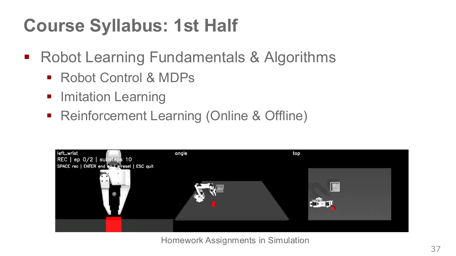
Control and Markov decision processes (MDPs) provide a basic language for robot–environment interaction. They make explicit the structure in which applying an action in the current state leads to a next state and a reward.
The SO-101 exercise introduced in the lecture takes control code learned in MuJoCo into a real-arm project with a similar interface. Shared joint numbering and command formats make reuse easier. Achieving the same result on hardware also requires checking friction, sensor calibration and control timing. ETH exercise repository
The course uses MuJoCo simulation assignments linked to the SO-101 arm. The environment code in official HW2 shows where observation generation, action handling, physics stepping and reward calculation connect. It is an assignment template with functions for students to complete.
The environment code separates display timing from physics and control timing. A 0.002-second physics step with each action held for 50 physics steps gives a 0.1-second action interval, or 10 Hz. Display FPS and policy-action update frequency are different quantities.
NVIDIA’s official Isaac Lab repository offers an extension. Its robot-learning environments and reinforcement-learning examples let us inspect how robot models, observations, actions and rewards are configured. The official documentation provides installation and environment examples. This chapter does not claim to have run Isaac Lab training.
At 56:55–58:26 of ETH Lecture 1, using the same arm in simulation assignments and the real project is explained through code reuse. What transfers is the observation–action interface and the structure of the control code. This does not make simulated friction, contact or sensor delays identical to reality. When a policy that passes simulation is evaluated on hardware, first check that the same commands represent the same physical quantities.
#P039 · Extending to generative models, world models and generalist policies
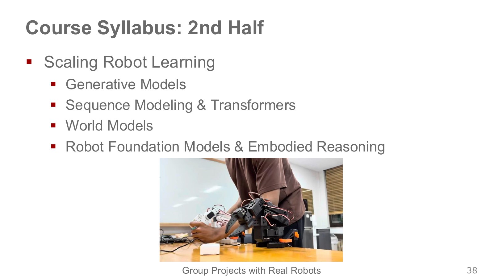
After understanding basic policies, we can broaden learning across tasks and datasets. Generative models can represent distributions of possible actions or trajectories, while Transformers provide a computational structure for relationships among observations and actions over time.
A world model predicts how the environment changes when an action is taken. Predicting the future also connects to planning: candidate actions can be compared before all of them are physically executed.
The next question is how to combine these concepts into one robot system. Distinguish each model’s role within the flow of understanding instructions, reading the scene, choosing actions and observing the results again.
Separate learning from planning here as well. Updating a predictive model from new execution experience is learning; computing and comparing candidate action outcomes using the current model is planning. DeepMind/UCL Lecture 1, 1:13:26–1:14:28 explains that a planner can exploit errors in a learned model. A shortest path through a passage that exists in the model but not in the real wall cannot be executed.
In the cup example, a contact model that underestimates gripper slip may lead a planner to conclude that a very weak grip is enough. Generating plausible-looking future video and predicting physics accurately enough to compare actions require different evaluation questions. World models are intended to reduce real trial and error, so we must check whether the planned outcome survives actual execution.
#P040 · From teleoperation to learned autonomous manipulation
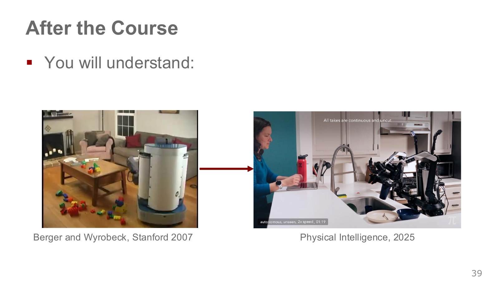
The 2007 PR1 on the left and the 2025 Physical Intelligence demonstration on the right share the goal of manipulating everyday objects. The change emphasized by the lecture is the move from human operators choosing actions in real time toward learned policies generating them.
Even when the tasks look similar, their data, robot structures, sensors and initial conditions differ. Read the comparison as an illustration of a direction of progress, distinct from a controlled experiment measuring one model’s improvement.
To understand an actual policy, look beyond the appearance of a demonstration to its training data, inputs, outputs and handling of failure.
#P041 · Observation, decision and action in autonomous driving
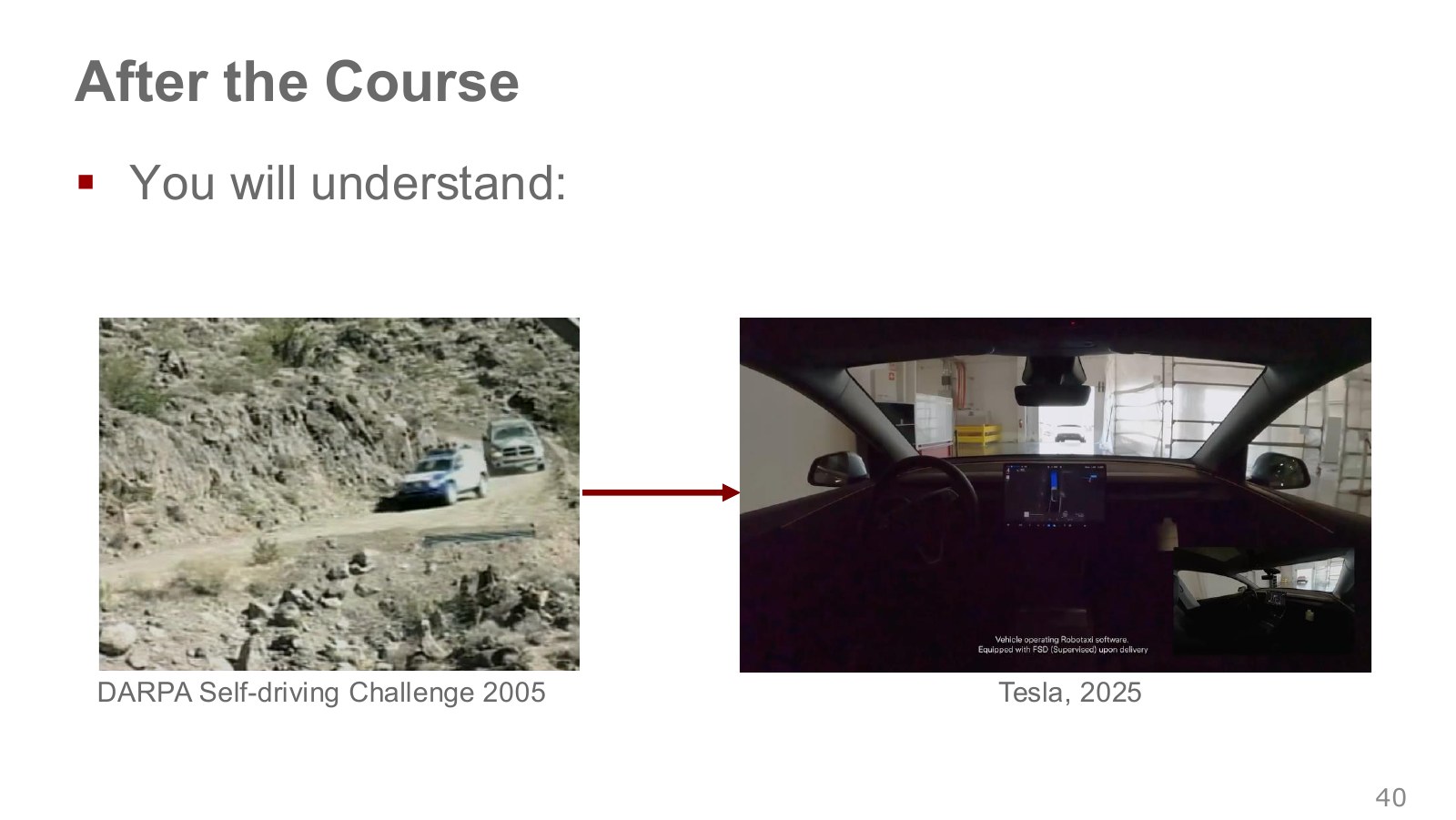
The slide contrasts the 2005 DARPA autonomous driving challenge with a 2025 Tesla demonstration. Moving a car and grasping an object with an arm are different tasks, but both involve sensing the surroundings, choosing actions and observing their consequences.
Perception of lanes and obstacles connects to prediction of other vehicles, planning a route ahead, and control of steering and acceleration. Which parts are learned and which use explicit models varies by system.
Checking operating conditions and the scope of human supervision, without extending one demonstration to autonomy on every road and in every condition, is also a useful approach to evaluating robots.
#P042 · Asking the same questions about humanoids
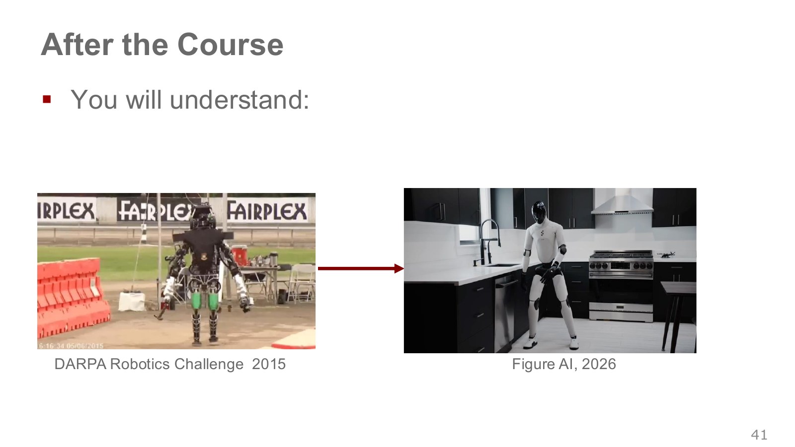
The robots of the 2015 DARPA Robotics Challenge and later Figure demonstrations show striking changes in movement and manipulation. A humanlike appearance and the tasks a robot can perform independently nevertheless need separate consideration.
Examining how a policy uses cameras and body state, how it learns from human demonstrations, and whether it can act on unfamiliar objects and arrangements tells us more than the smoothness of its movements alone.
Low-level balance control, manipulation through contact and planning a multistep task are connected but distinct problems. Separating these layers reveals a model’s role in a general-purpose robot system.
#P043 · From large-model reasoning to bodily control
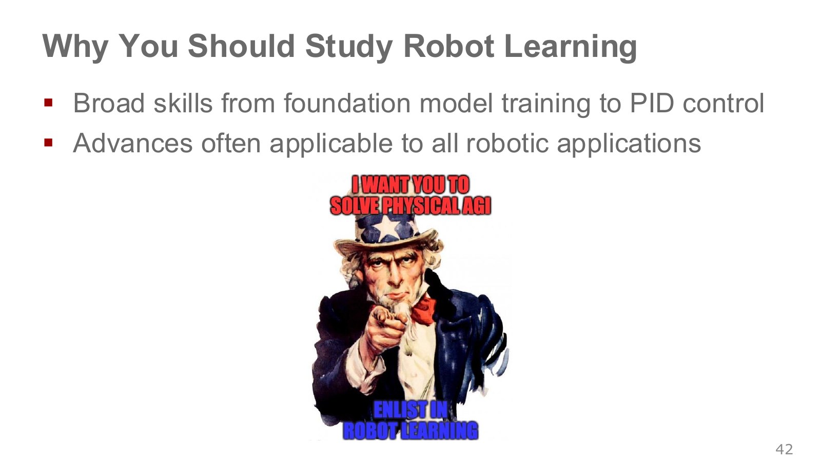
Robot learning spans high-level representations and reasoning in foundation models through to low-level control of motors. It brings fields together because cameras, data, models, control and hardware all need to be understood in relation to one another.
The questions to carry from this chapter are simple: What does the robot observe, what actions does it produce, what signal does it learn from, and in what environment is it evaluated? These four questions apply when reading papers and code for arms, mobile robots, autonomous driving and humanoids alike.
The next chapter uses control and MDPs to express robot–environment interaction in more concrete mathematical terms.
#Continue with code
To first explore the effect of reusing observations, try the feedback example I ran. It uses Python’s standard library to compute one-dimensional positions with a speed limit.
cd docs/robot-learning/labs/01-feedback-loop
python3 -m unittest -v
python3 feedback_loop.py --out results
With a single +0.4 m position disturbance, the final open-loop error after 60 steps was 0.4 m, while the feedback error was about 8.92×10⁻⁷ . These are computed results for the specified one-dimensional model. The example illustrates the effect of using new observations during execution, rather than updating a policy through learning. See the exact results alongside the execution and checking instructions.
For robot-arm physics simulation, continue with the ETH MuJoCo assignment. For a wider range of robot-learning environments, explore NVIDIA Isaac Lab and its official documentation.
#Sources
- Oier Mees — Robot Learning: From Fundamentals to Foundation Models, ETH Zurich, Lecture 1 · Lecture video
- Lecture-slide image source · Attribution guide
- Hado van Hasselt — DeepMind × UCL, Introduction to Reinforcement Learning (2021) · Original slides
- Hung-yi Lee — NTU ML 2021: RL Basics · Imitation Learning · Official course index · Original PPTX
- RT-2: Vision-Language-Action Models · Open X-Embodiment
- DAgger — A Reduction of Imitation Learning and Structured Prediction to No-Regret Online Learning
- SRI — Shakey the Robot
Lecture and slide copyright: Oier Mees and the respective rights holders. Photographs, videos, paper figures and trademarks included in the slides belong to their original rights holders. These notes introduce the course materials with attribution, adding explanations originally written in Korean and separate code examples. P numbers follow the file order in the slide-image source.