A hand paused in front of a cup could be approaching to grasp it or withdrawing after a failed attempt. A robot needs not only the current scene but also the process leading to it. This chapter represents that process as a sequence and connects relevant information through attention.
Oier Mees · ETH Zurich 2026, Lecture 7 · Official lecture · Original PDF
#P002 · From one photograph to actions unfolding over time
Chapter 06 represented distributions of possible actions with VAEs, diffusion, and flow matching. Here, we examine how to divide data into units and structure relationships between past information and future actions. Generation methods and sequence architectures are compatible design choices. Transformers need not operate autoregressively; they can also be used within diffusion or flow models.
A sequence is an ordered collection of data, such as words in a sentence, video frames, or joint commands over time. A token is a unit the model processes, and an embedding represents it as a numerical vector. Language tokens usually map from integer vocabulary indices to vectors. Image-patch or continuous-action tokens may already be continuous vectors. Treating everything as tokens does not mean converting every input into the same kind of integer.
The lecture moves from language-model principles to vision–language models (VLMs), then vision–language–action models (VLAs). Let us examine the connections needed between predicting token indices and achieving goals in the physical world.
#P003 · Can the current scene alone reveal the direction of motion?
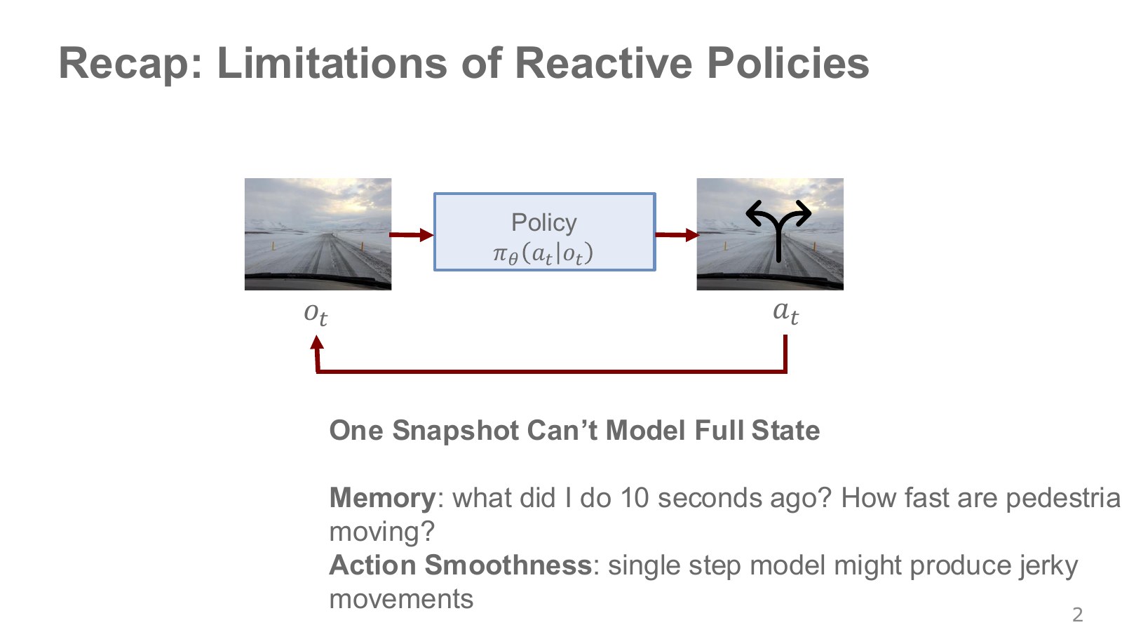
A policy sits between an icy-road photograph and three branching arrows. This is a reactive policy selecting the next action from the current observation alone. But a pedestrian at the same photographed location may require different responses depending on whether they are approaching or moving away from the car. Previous positions and time intervals allow velocity estimation.
Likewise, a car at the same position on an icy road may require different actions depending on whether it is sliding or stationary. A still image shows position; observations over time provide clues about speed and direction. Inferring the current state from history and producing smooth future commands are separate problems.
Another issue is action continuity. Independently choosing an approach direction each moment can make the hand oscillate between left and right. Using past information and generating consistent future commands are related but distinct: one concerns observation memory, the other output action-sequence design.
A reactive policy can be appropriate when one observation already contains sufficient state information or the task is simple. The figure does not claim that every single-time-step policy fails; it asks whether one sensor snapshot contains enough information for the decision.
#P004 · Under partial observability, consider both past observations and actions
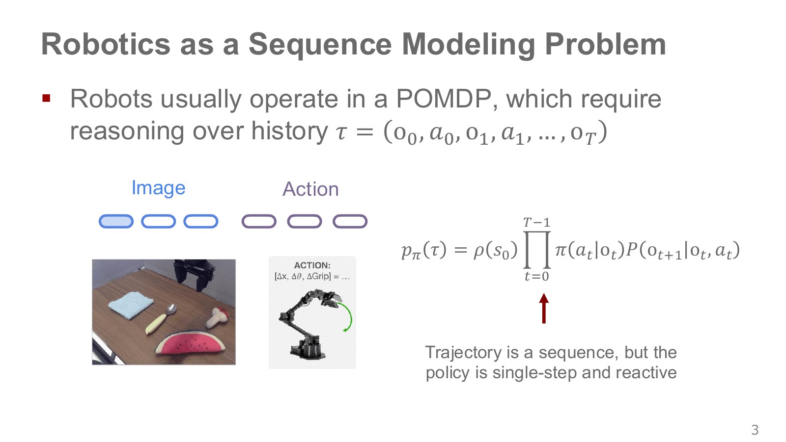
The table photograph represents the current visible scene, and the robot illustration represents actions affecting it. The physical state includes information a photograph cannot fully reveal, such as occluded objects, contact states, and velocity. This can be modeled as a partially observable Markov decision process (POMDP). Even if world states are Markovian, observation images alone need not be.
Explore the symbols and calculation A policy conditioned on observation and action history
Read the equation in words
Collect scenes observed and actions actually taken into a history, then use it as input to the policy selecting the next action.
Understand each symbol
- The sensor observation at step . It is not assumed to equal the full physical state.
- The action chosen at step : for example, a torque, a joint target or a movement direction, depending on the setup.
- The parameters collecting the trainable weights of the network or policy.
- Observation–action history through the current observation. The current action has not yet been appended.
- A placeholder leaving the particular action value in the distribution unspecified.
- Conditional notation: the information to the right of the bar is given. This is not a division sign.
Follow the calculation
- List observations and actions in their order of occurrence.
- Condition the next-action distribution on history including the current observation.
Check with a small example
Seeing the initial photograph, the gripper-closing action, and the subsequent photograph together can help assess grasp success better than the current photograph alone.
An illustrative example for understanding the equation.
Here, denotes observations, actions, and the history so far. For example, knowing a previous command closed the hand can help interpret the current finger configuration and object position. Feeding history into a network does not guarantee exact reconstruction of hidden state; unseen information remains uncertain.
The slide’s compact trajectory-probability equation summarizes the earlier reactive policy. Assuming that current observations and actions suffice to predict the next observation adds an assumption in a general partially observed problem. Retaining observation history gives the following expression.
Explore the symbols and calculation Probability of an observation–action sequence with history retained
Read the equation in words
Calculate sequence probability while retaining possible dependence of the next observation on past history. Do not assume the current observation alone is the state.
Understand each symbol
- The sensor observation at step . It is not assumed to equal the full physical state.
- The action chosen at step : for example, a torque, a joint target or a movement direction, depending on the setup.
- The parameters collecting the trainable weights of the network or policy.
- One trajectory containing states and actions in time order. This symbol does not denote an angle.
- The length of a trajectory or sequence. Here it sets how many steps enter the sum or product.
- The accumulated history of observations and actions.
- The next-observation distribution given the full history and current action.
- Multiply every term in the indicated range. This appears when computing the joint probability of successive choices.
- Conditional notation: the information to the right of the bar is given. This is not a division sign.
Follow the calculation
- Start with the first observation's probability.
- Successively multiply history-conditioned action and next-observation probabilities.
Check with a small example
Even identical photographs can lead to different next-image distributions if the preceding motion directions differ. This expression retains that distinction through history conditioning.
An illustrative example for understanding the equation.
Instead of retaining the entire history, one can update a belief—a probability distribution over hidden states—or use a learned summary vector. Sequence models learn these summaries and references from data.
#P005 · An autoregressive model predicts the next element from the preceding sequence
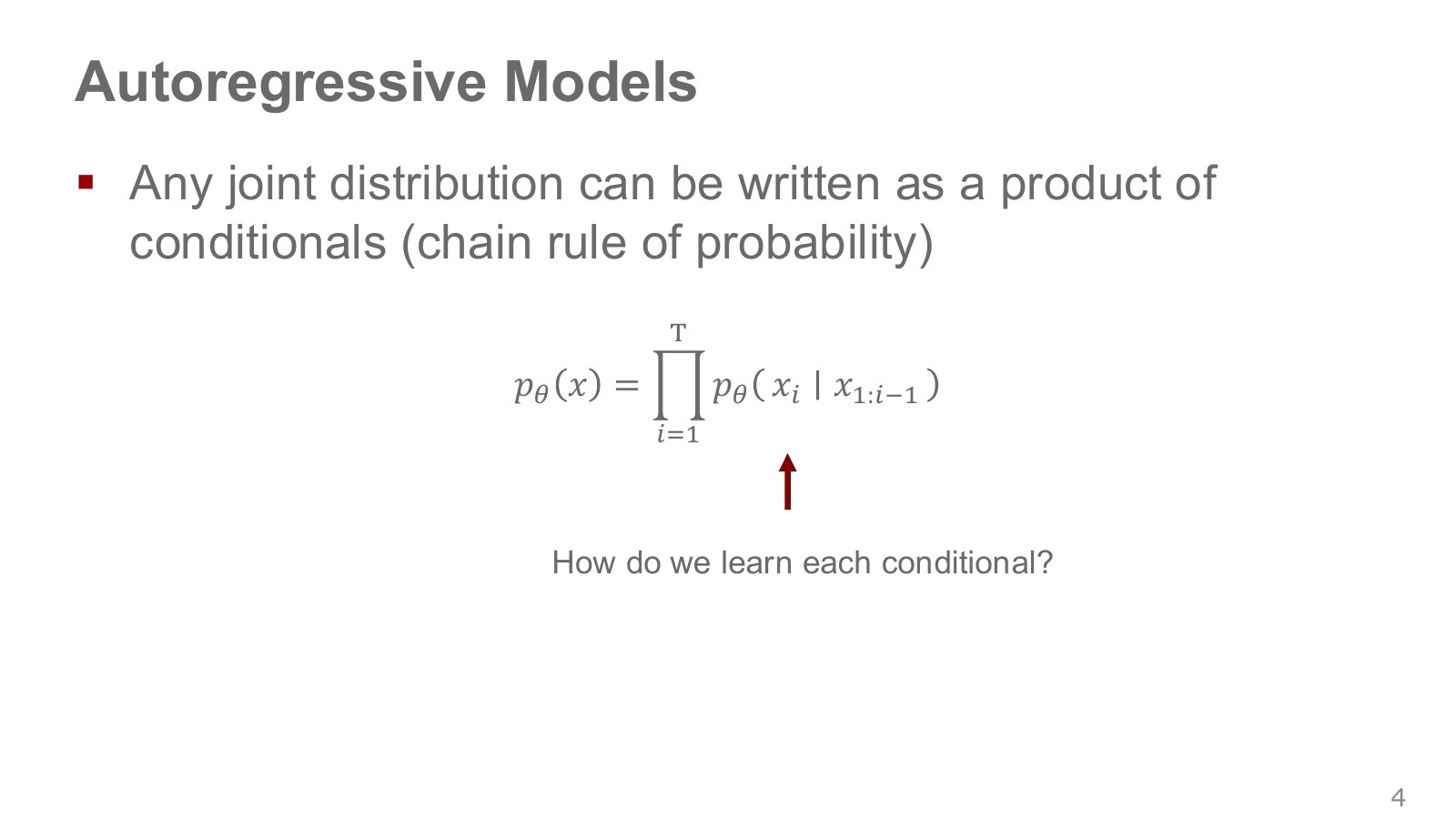
Imagine extending a sentence one word at a time. Select the first token, use it to select the second, and continue conditioning on all tokens generated so far. This generation procedure, using earlier outputs as subsequent inputs, is autoregression.
Explore the symbols and calculation A joint distribution factored by the probability chain rule
Read the equation in words
The probability of a full token sequence is the product of each next-token probability given its prefix. There is no assumption that the last token sees only one preceding token.
Understand each symbol
- The parameters collecting the trainable weights of the network or policy.
- The length of a trajectory or sequence. Here it sets how many steps enter the sum or product.
- The th token and all preceding tokens.
- Multiply every term in the indicated range. This appears when computing the joint probability of successive choices.
- Conditional notation: the information to the right of the bar is given. This is not a division sign.
Follow the calculation
- Specify the first token.
- Condition each next-token probability on all tokens so far and multiply to the end.
Check with a small example
Conditional token probabilities 0.5, 0.8, and 0.2 give sequence probability 0.08. This computes a long sentence's probability from smaller factors.
An illustrative example for understanding the equation.
The factorization itself is the probability chain rule and requires no Markov assumption. How much to remember, and for how long, is a modeling choice for each conditional distribution. Even if abbreviated notation appears to reference only one preceding token, the main text conditions on the entire prefix .
Robots can form sequences from observations, actions, language, and other information. But generating future environment observations differs from generating only actions given observations. Using a sequence model does not necessarily make it a world model predicting future video.
#P006 · An RNN repeatedly updates a fixed-size memory vector
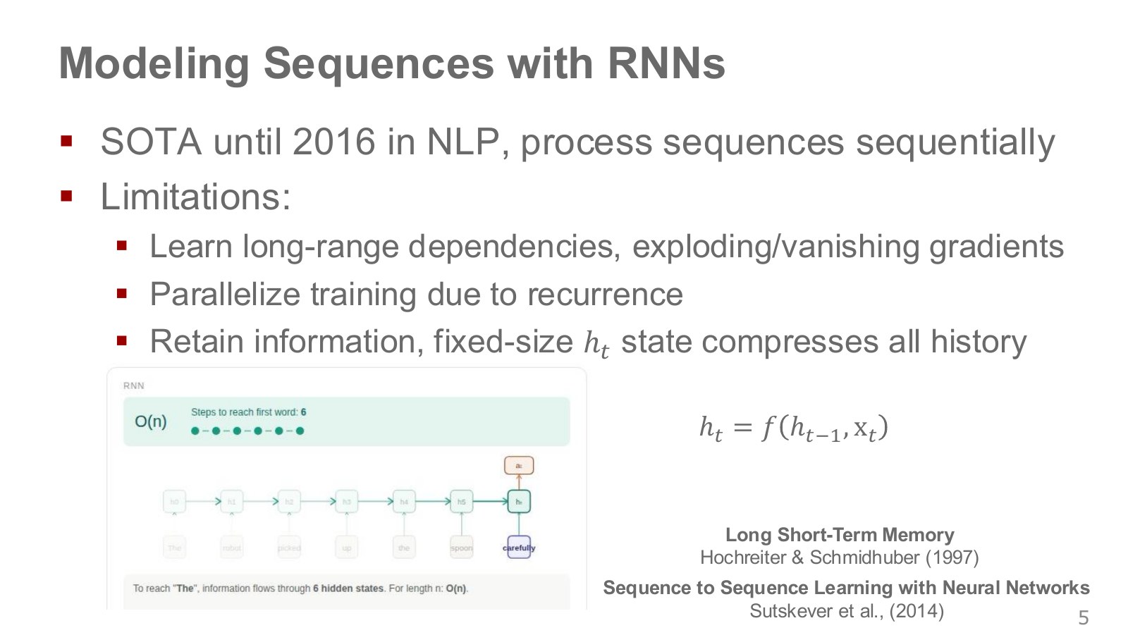
The small boxes along the bottom show the same network unrolled over time. A recurrent neural network (RNN) forms its next memory from its previous memory and new input. It shares weights across time, rather than creating a different model at each step.
Explore the symbols and calculation Updating an RNN's hidden representation
Read the equation in words
An RNN combines a memory vector summarizing the past with the incoming input to form a new memory. It updates a fixed-length numerical representation rather than storing the full history unchanged.
Understand each symbol
- The previous and current hidden-memory vectors: learned summaries, not directly human-labeled states.
- The current input vector, such as a token or observation.
- A learnable memory-update function.
- The parameters collecting the trainable weights of the network or policy.
- Here, the input-reading order. The subscript does not identify a vector component.
Follow the calculation
- Pass the previous memory and new input together into the transformation.
- Store the new memory for the next step. The transformation's weights are shared across time.
Check with a small example
For an illustrative update , previous memory 2 and new input 3 give new memory 4. Actual RNNs usually use vectors and nonlinear functions.
An illustrative example for understanding the equation.
Here, is a hidden memory vector summarizing information read through time . The previous memory is , the new input is , and is a learned function combining them to update memory. Memory components do not have predefined meanings such as joint angles; they are internal features learned to aid prediction. Distinguish this vector from the full raw history introduced earlier. Updating a fixed-size vector accommodates variable-length inputs while keeping runtime memory compact.
For distant information to affect the current training error, however, it must pass through many updates. Repeated multiplication of derivatives can cause vanishing or exploding gradients. LSTMs mitigate this with gates controlling retention and deletion. Temporal training parallelism is also limited because the previous memory is needed before calculating the next. This is not simply a consequence of autoregression: Transformers can also generate autoregressively.
#P007 · Attention directly connects distant tokens
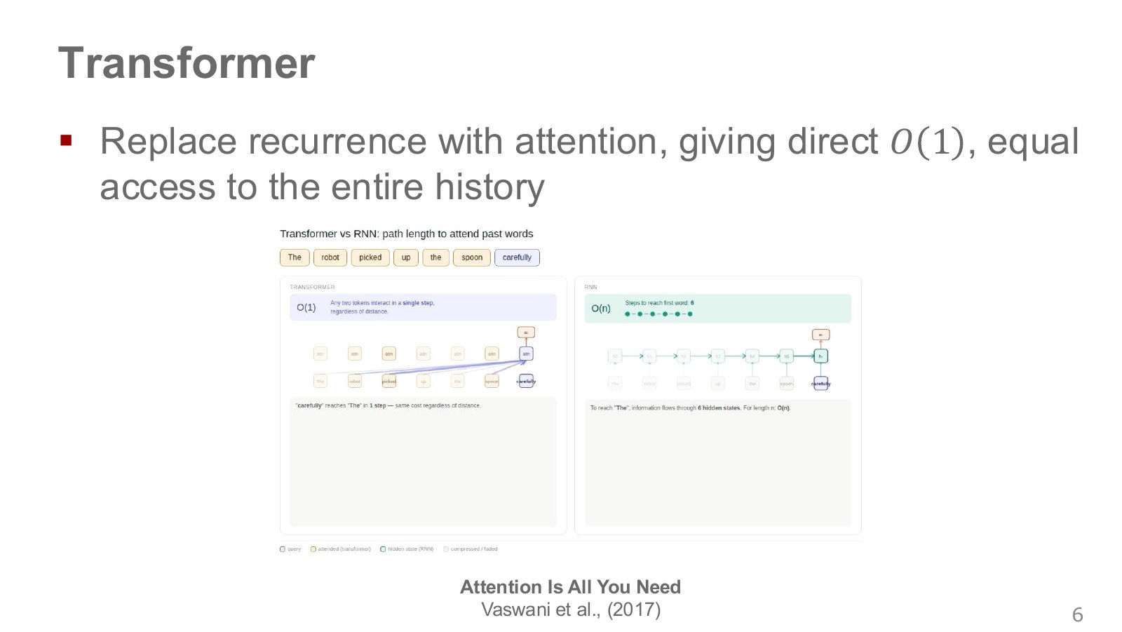
The figures compare paths by which the last word references earlier words. An RNN passes through successive intermediate memories, while self-attention directly compares token representations entering the current layer. Its advantage is a shorter connection path between distant positions.
The slide’s refers to path length between positions. It does not mean total attention computation remains constant as sentences grow. Standard dense attention compares every position pair, requiring computation proportional to the square of token count.
Direct connections do not guarantee perfect long-context understanding or unlimited memory. Context windows, model capacity, position information, and training data remain limiting factors. Transformers offer a useful structure for learning long-range relationships rather than automatically solving every long-range dependency problem.
#P008 · Queries and keys determine weights; values supply the information to combine
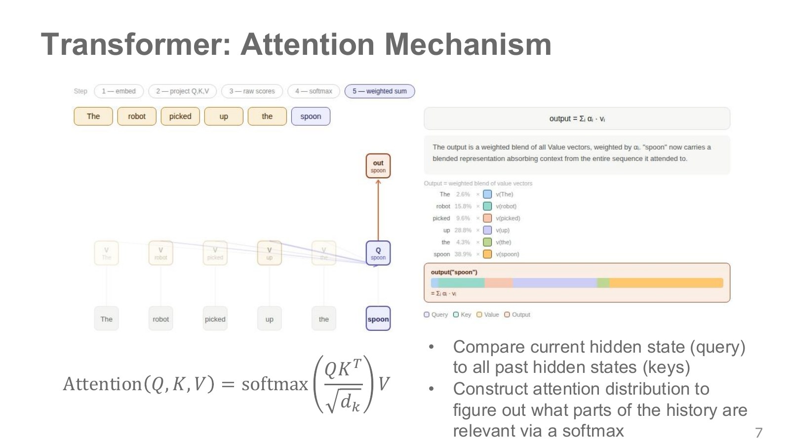
The figure shows the final token, spoon, referencing other words to form a new representation. Each token produces three vectors. A query expresses information sought; a key is a representation used for comparison; a value contains information to pass along. Think of comparing a search query with identifying labels, then gathering the associated content.
Explore the symbols and calculation Projecting token representations into queries, keys, and values
Read the equation in words
Create separate representations for information sought, comparison labels, and content to transmit from the same input tokens. Three learned matrices serve these different roles.
Understand each symbol
- A matrix with one token's input representation per row.
- Three projection matrices learned separately.
- The query, key, and value matrices. Here, does not denote reinforcement-learning action value.
Follow the calculation
- Collect token vectors as rows of an input matrix.
- Multiply the input by each of three weight matrices to obtain queries, keys, and values. Each output component sums products of corresponding elements from an input row and weight column.
Check with a small example
Three tokens with input dimension 4 and key dimension 2 give a 3×2 query matrix. Representation dimension changes, not token count.
An illustrative example for understanding the equation.
Explore the symbols and calculation Scaled dot-product attention
Read the equation in words
Dot products between queries and keys give reference scores. Normalize them rowwise like probabilities, then combine values to determine what information to retrieve from where.
Understand each symbol
- The query, key, and value matrices. A query–key dot product multiplies corresponding vector components and sums them into one comparison score.
- The transpose exchanging key rows and columns, and the key dimension—the number of vector components. Dividing by its square root moderates score growth with dimension.
- A mask assigning zero to permitted connections and negative infinity to blocked ones.
- The new representation each query obtains by combining values.
- Divide each exponentiated score by the sum of exponentiated scores to give positive rowwise weights summing to one. Exponentiation raises approximately 2.718 to the score.
Follow the calculation
- Divide dot-product scores by the square root of key dimension and add the mask.
- Use each query's softmax weights to form a weighted average of value rows.
Check with a small example
Scores 0 and 1 give weights approximately 0.269 and 0.731. Values 2 and 6 then give output approximately 4.924.
An illustrative example for understanding the equation.
Each row of represents one token. Three learned matrices produce vectors with different roles from the same input. The dot product of and gives a comparison score, divided by the square root of key dimension to moderate dimension-dependent magnitude. Softmax converts each query row’s scores into nonnegative weights summing to one. The final multiplication forms a weighted sum of values. Colored bands on the right show how much each value contributes.
The mask blocks disallowed connections and is zero where there is no restriction. For example, two key scores of 0 and 1 give softmax weights approximately 0.269 and 0.731. This does not mean the second word has a 73.1% probability of being important in the real world. These are internal information-mixing weights, not automatically causal explanations or object-detection probabilities.
Stanford CS25, 23:38–28:12 explains this as information passing between nodes. NTU’s self-attention lecture, 24:57–30:03 separately walks through comparison scores and weighted value sums. Multiple heads perform references in parallel with different weights; stacking layers adds sequential depth that reprocesses their outputs.
#P009 · Tell the model where a token is, as well as what it is
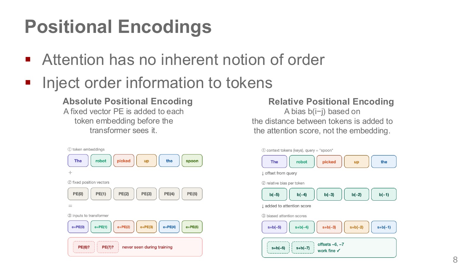
“The robot picked up the spoon” and “The spoon picked up the robot” contain the same words but mean different things. Without position signals or order-dependent masks, basic self-attention is permutation-equivariant: rearranging inputs rearranges outputs in the same way. Content comparisons alone cannot adequately distinguish order.
Absolute position representations on the left add position vectors to token embeddings. Relative representations on the right adjust comparison scores according to query–key separation. A separation of four positions remains the same if the whole sentence shifts.
Explore the symbols and calculation Attention scores with relative-position bias
Read the equation in words
Add a correction based on positional separation to the content-comparison score. Even identical words can be referenced differently at different relative positions.
Understand each symbol
- The query vector at position and key vector at position .
- The attention score between the two positions.
- A bias added according to relative distance.
- The key vector's dimension.
Follow the calculation
- Calculate the token representations' dot-product score.
- Pass the difference between position indices into the bias function and add it to the score.
Check with a small example
Content score 0.6 and bias −0.2 for a two-position separation give final score 0.4.
An illustrative example for understanding the equation.
Absolute position methods include fixed sine/cosine signals and learned tables; relative methods also take multiple forms. Relative positions can help with longer inputs than those seen in training, but do not guarantee perfect generalization to arbitrary lengths. Unseen distances, training lengths, and changes in attention distributions still matter. Read the long-sequence checkmark as the design’s intent.
#P010 · The encoder reads inputs; the decoder generates an answer not yet available
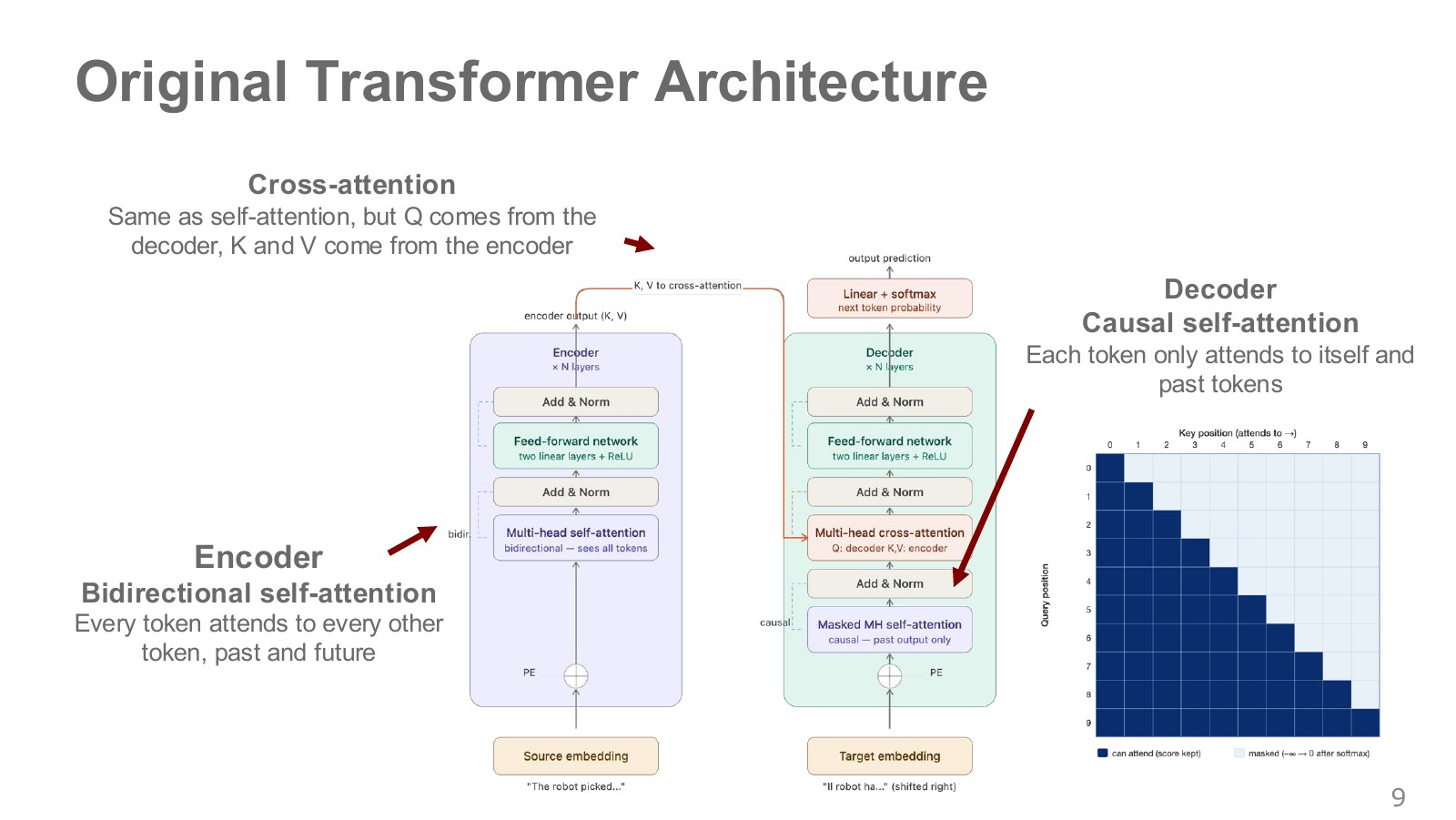
The two middle columns are the original translation Transformer’s encoder and decoder. The encoder receives the entire source sentence, so tokens may refer to source positions on either side. The decoder generates a translation and cannot see future translated tokens. The lower-right triangle depicts permitted references: rows query positions and columns referenced positions, with only the diagonal and lower-left region open.
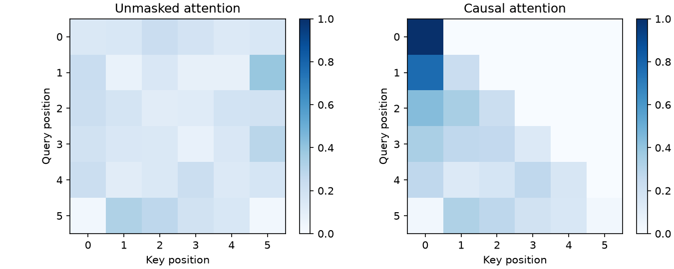
A causal mask adds negative infinity to future-position scores, making their post-softmax weights zero. “Causal” here means respecting generation order, not automatically recognizing real-world causes and effects. It also differs from a padding mask, which hides empty tokens inserted to align sequence lengths.
In cross-attention, queries come from the decoder and keys and values from encoder outputs. It asks which part of the source to reference when extending the translation produced so far. In self-attention, all three vectors come from the same sequence.
The feed-forward network nonlinearly transforms features at each position. Add introduces the previous representation to preserve information and derivative paths. Norm normalizes feature magnitudes. The information gathered by multiple heads is repeatedly combined with this processing. A full Transformer is not just one weighted averaging of values.
#P011 · Training provides the correct prefix and computes every next-token loss
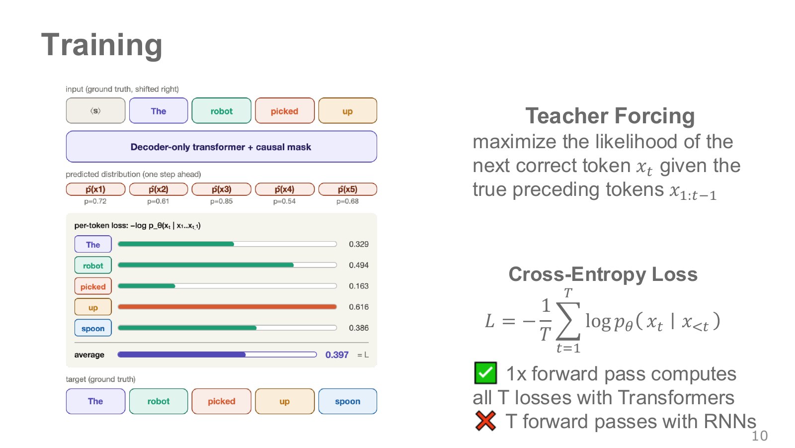
The top input row shifts the target sentence one position to the right. After the start token, The is supplied to predict robot; each position receives the correct preceding tokens. This is teacher forcing, distinct from immediately feeding the model’s own incorrect word back as the next training input.
Explore the symbols and calculation Negative log likelihood of the correct next token
Read the equation in words
Minimize average negative log probability to give correct next tokens higher probability. During training, each position conditions on the correct preceding tokens.
Understand each symbol
- The parameters collecting the trainable weights of the network or policy.
- The length of a trajectory or sequence. Here it sets how many steps enter the sum or product.
- The current target token and the correct tokens preceding it.
- The mean negative-log-likelihood loss.
- Add every term over the indicated range, computing one term and repeating through the end of the range.
- The natural logarithm. It converts products into sums and is defined only for positive inputs.
- Conditional notation: the information to the right of the bar is given. This is not a division sign.
Follow the calculation
- Read the correct token's probability at each position.
- Negate its natural logarithm and average across sequence length.
Check with a small example
Correct-token probabilities 0.5 and 0.25 at two positions give mean loss approximately .
An illustrative example for understanding the equation.
Higher probability on the correct token yields lower loss. Target probability 0.8 gives loss approximately 0.223; 0.01 gives approximately 4.605. This matches cross-entropy for one discrete target. Models trained only on robot action tokens can mask losses on observation and instruction tokens.
Because the correct sentence is already available, a causally masked Transformer can calculate losses at multiple positions in one batched forward pass. Actual generation remains sequential because each next token depends on earlier generated outputs. Parallel training does not mean generation finishes in one pass. At execution, the model’s own errors enter subsequent inputs, creating another mismatch with training.
#P012 · Choosing token units between characters and words
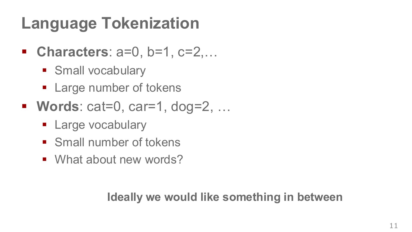
Character indices give a small vocabulary but turn long sentences into many tokens. Word indices shorten sequences but enlarge the vocabulary and make new words difficult to handle. For example, robot, robots, and robotic could be separate words, or share robot as a common part with separate endings.
A vocabulary is the list of available tokens. Token-index magnitudes usually do not encode an ordering of word meanings. An index retrieves a row from an embedding table, whose vector is adjusted during learning to form useful representations.
Tokenization is not only about semantics. Longer sequences increase attention comparisons and generation steps. How to represent the same information compactly and reliably reappears later in robot-action compression.
#P013 · BPE repeatedly merges frequent neighboring tokens
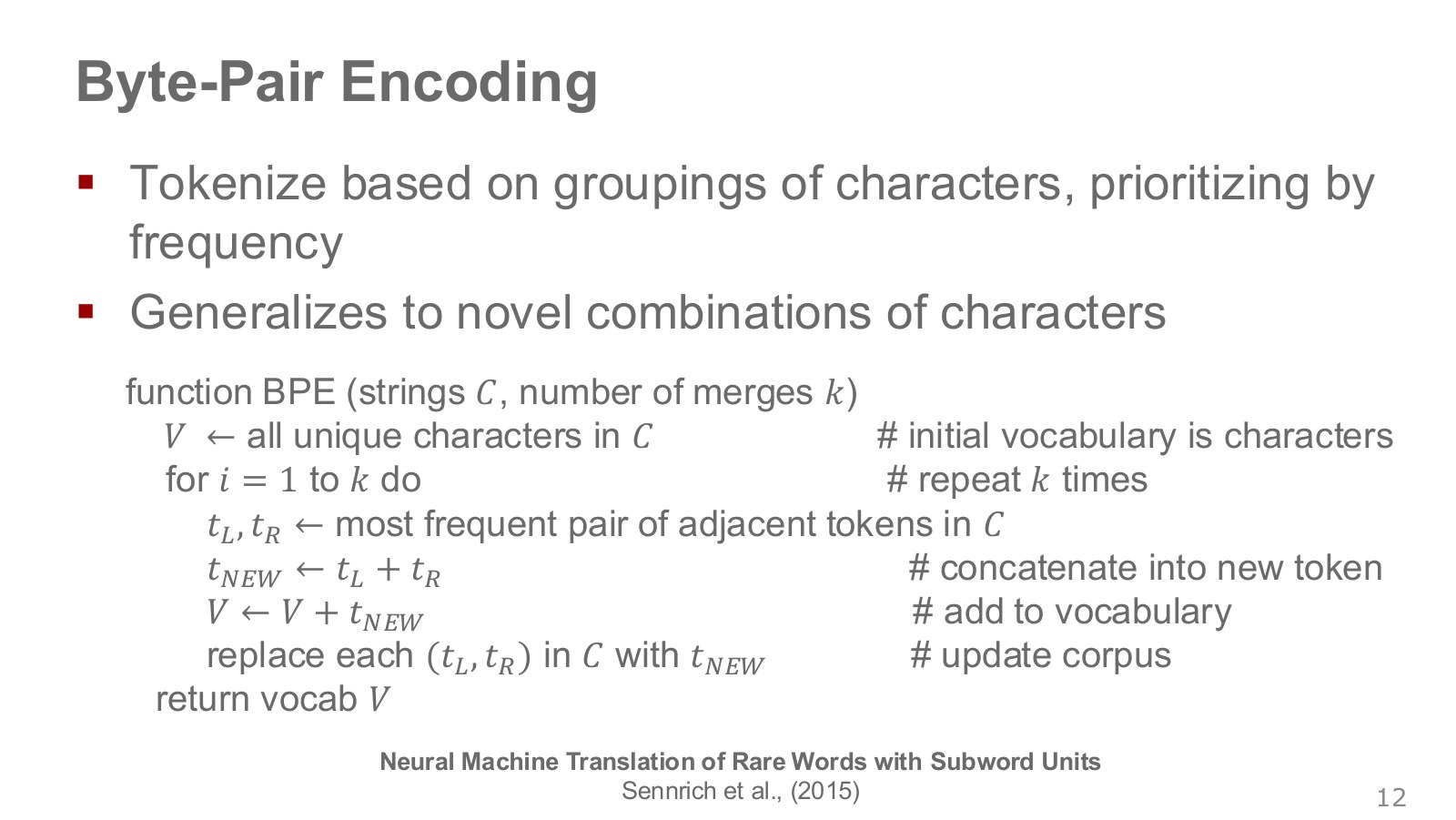
Begin by dividing data into small symbols such as characters. Find the most frequent consecutive token pair across the training corpus and merge it into one new token. Repeat until reaching the desired vocabulary size. Merge rules are learned during training and reused when encoding new sentences.
For example, frequent neighbors r and o can merge into ro; frequent ro and b can then form rob. Each merge preserves the original symbol sequence. Because it can be decoded back to those symbols, fewer tokens do not necessarily mean lost sentence information.
The original subword BPE paper explains representing rare words using known smaller units. Handling symbols absent from the initial alphabet is a separate matter. Byte-level representations, introduced later, provide a more comprehensive base symbol set.
#P014 · Distinguishing token-count reduction from file-size reduction
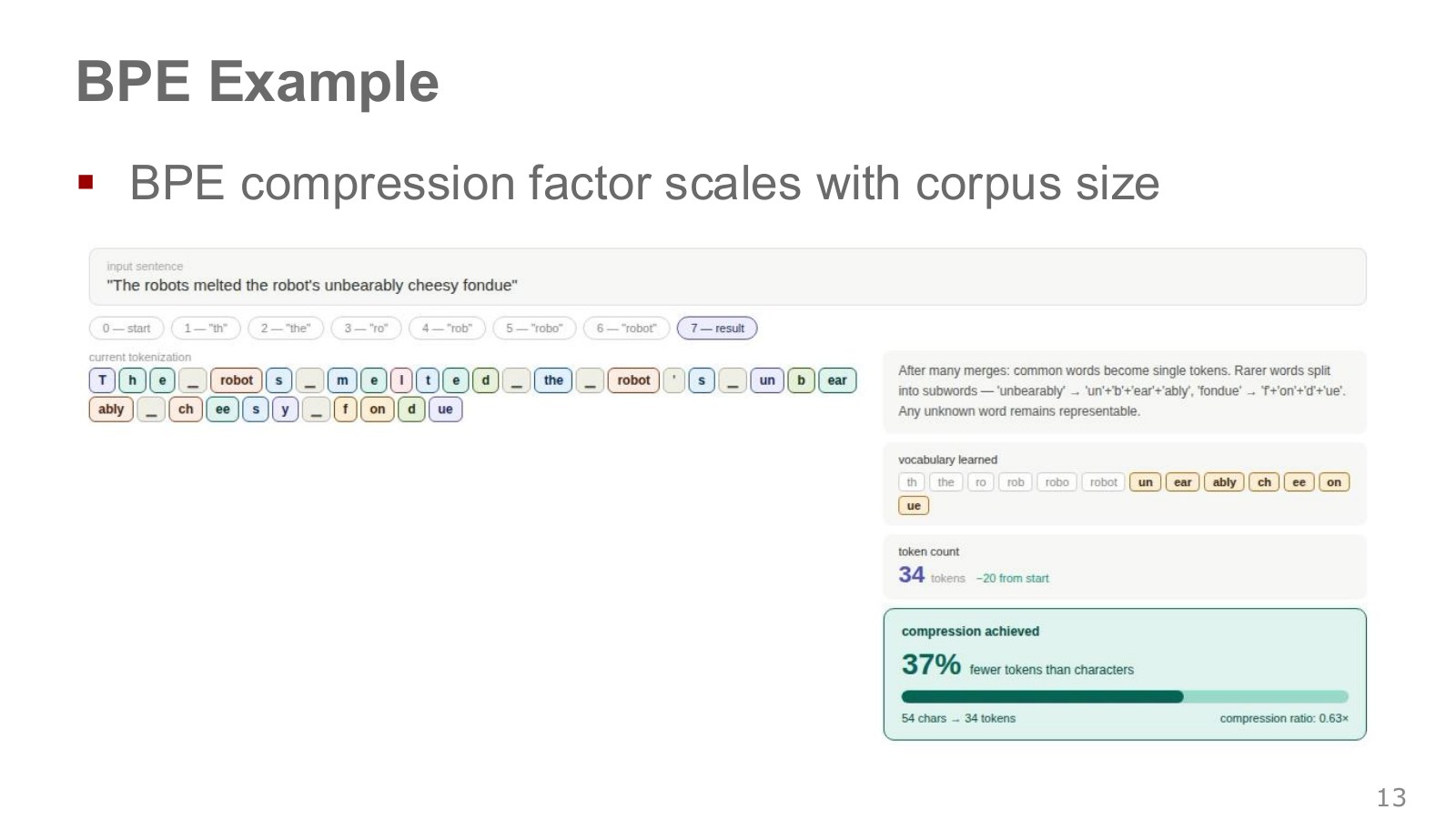
As merges proceed, frequent substrings in the example sentence become larger units. The reduction from 54 characters to 34 tokens compares counts in this example. It does not mean the disk file becomes exactly 37% smaller, because bits per stored token index and vocabulary size also matter.
Larger corpora can improve estimates of frequent patterns, but do not guarantee better compression for every input. Language, spacing, symbols, vocabulary size, and training distribution all matter. These choices also help explain differing token counts for Korean sentences and English code.
Our small character-BPE implementation likewise shortens repeated strings and reconstructs their original text. It does not reproduce a commercial language model’s actual tokenizer; it implements only the merge rules needed to demonstrate the principle.
#P015 · Architecture, position representations, and memory computation for long sequences
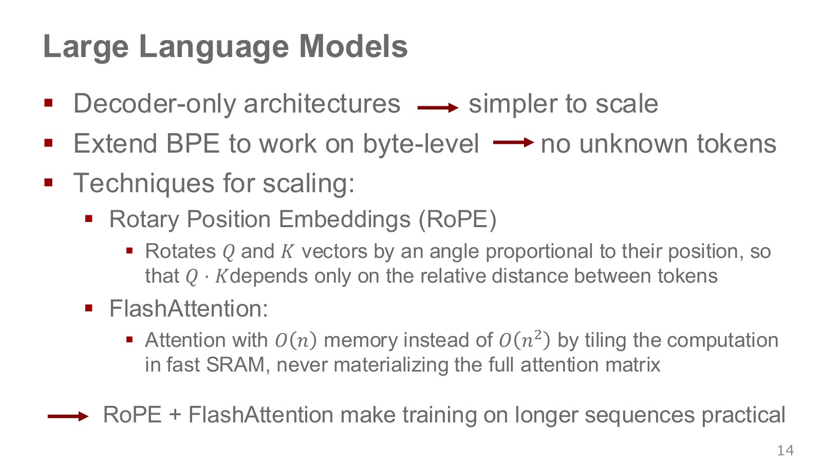
First, decoder-only models handle input context and output sequences within one generative model, without the original translation architecture’s separate encoder. This is important in GPT models, but not universal to language models. Second, byte-level tokenization uses raw bytes as base symbols, representing new characters through their byte sequences. Representability does not imply semantic understanding.
Third, RoPE rotates coordinate pairs in queries and keys by position-dependent angles. This makes the positional effect in their dot product depend on relative separation. Content vectors still affect the dot product, so distance alone does not determine the full score. Long-sequence generalization remains a separate challenge. RoPE paper.
Fourth, FlashAttention tiles computation into small blocks and reduces memory transfers instead of storing the entire token-pair weight matrix in large memory at once. It computes the required attention exactly, unlike sparse attention that omits selected comparisons. Even if storage for attention computation becomes linear at fixed head dimension, total dense-attention arithmetic does not become linear. FlashAttention paper.
Long-context support results from architecture and training conditions together. Adding RoPE and FlashAttention alone does not automatically guarantee memory accuracy or real-time control latency.
#P016 · Pretraining, fine-tuning, and in-context learning involve different changes
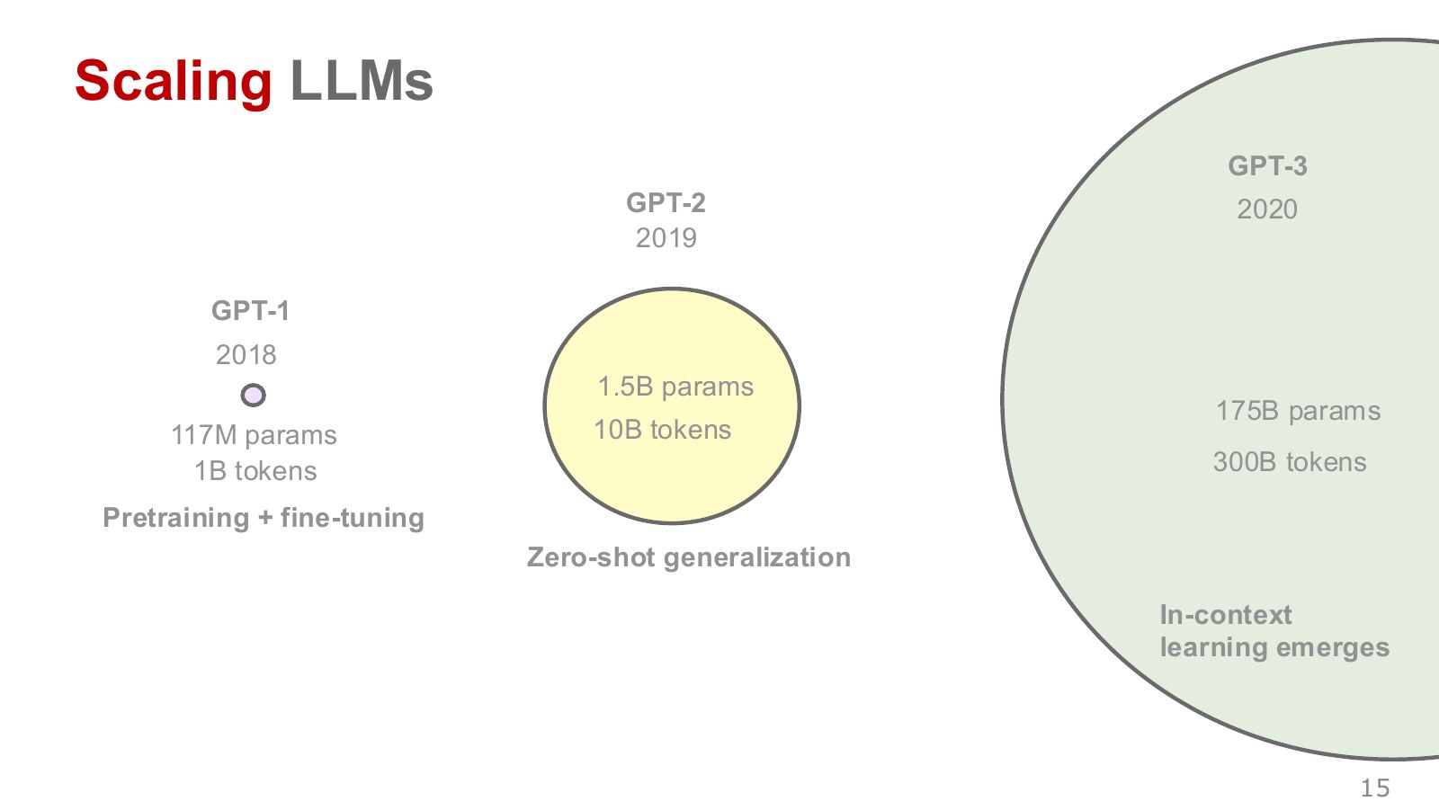
The circles of increasing size compare historical GPT model scales. Parameters are weights adjusted during learning; training tokens measure the amount of data consumed. More parameters do not automatically mean more training data.
Pretraining learns general representations and prediction capabilities from broad data. Fine-tuning subsequently updates weights for particular data or objectives. In-context learning supplies examples in a prompt to elicit a matching response pattern, without ordinary weight updates during that execution.
Zero-shot means no separate demonstration examples are included in the request; few-shot includes a small number. Neither means the model had no pretraining data. Experiments showing larger models using examples better are distinct from claims that increasing scale suffices for every task.
The lecture highlights GPT-3’s 175 billion parameters and 300 billion training tokens. The first describes weight count; the second describes textual units consumed during training. In a few-shot setup that provides three translation examples before asking for a fourth, those prompt examples do not retrain the weights. The observation concerns how differently scaled models use patterns in context. For robots, likewise record model size, demonstration volume, and demonstrations in the current context as separate axes. Original GPT-3 paper
#P017 · The graph compares effects of model size and the number of in-context examples
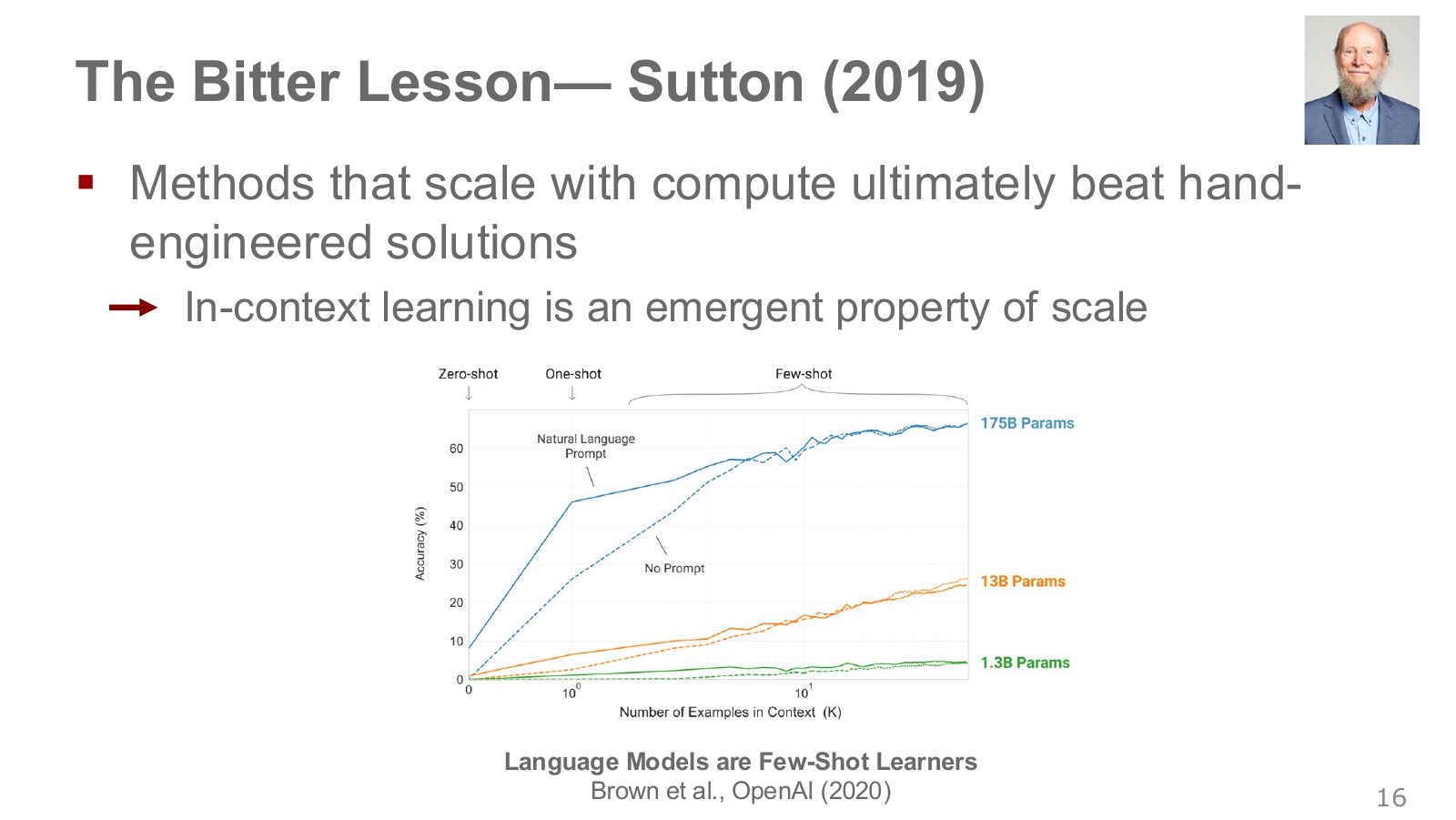
The person on the left is reinforcement-learning researcher Richard Sutton. The Bitter Lesson argues from historical examples that general methods exploiting computation have achieved strong long-term results. It can be read as cautioning against limiting scalability through current hand-engineered knowledge, rather than demanding that people design no structure at all.
The horizontal axis counts in-context examples; the vertical axis is accuracy in that experiment. Curve colors distinguish model sizes and show larger models making better use of examples in this setting. Accuracy in the cited language experiment is not a robot’s physical success rate.
For robots, the questions are concrete: which sensors and actions will be recorded, how much data will be collected, how will units be aligned across robots, and will greater computation fit the control cycle? Scale does not replace these design choices; it asks whether they can grow effectively.
#P018 · Divide the training-compute budget between model size and data volume
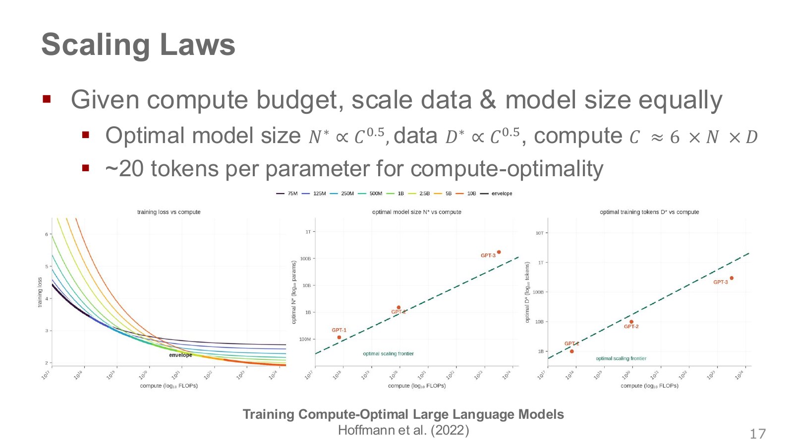
The curves on the left show how loss falls with more computation at each model size. The largest model does not always give the lowest loss for a fixed budget. An oversized model may be undertrained; an undersized one may reach capacity limits despite more data. The curves’ lower envelope connects favorable choices at different budgets.
Explore the symbols and calculation Approximate dense-language-model training compute and Chinchilla-style allocation
Read the equation in words
An approximate relationship for scaling model size and training data together under a compute budget, not a universal law for every architecture or cost category.
Understand each symbol
- Approximate training computation.
- Model-parameter count and training-token count. Here, is not a sample-mean count.
- Favorable scales under the compute budget and proportionality notation.
Follow the calculation
- Multiply parameter and training-token counts to approximate training compute.
- Under this scaling approximation, allocate both sizes according to the square root of the compute-budget increase.
Check with a small example
Quadrupling the compute budget doubles both model and data sizes under this approximation. Actual memory and inference latency do not enter this equation directly.
An illustrative example for understanding the equation.
Here, is parameter count, training-token count, and training computation. The two graphs on the right show favorable model and data sizes increasing together with the budget. Roughly following this relation, quadrupling compute doubles both model size and data volume.
Approximately 20 tokens per parameter is an empirical training-compute guideline from the Chinchilla paper’s setting, not a universal law for every language, model, or objective, nor a formula for robot demonstration counts. Attention overhead, inference cost, and data quality also matter alongside this dense-model approximation.
#P019 · Conditions for extrapolating small-experiment trends to larger runs
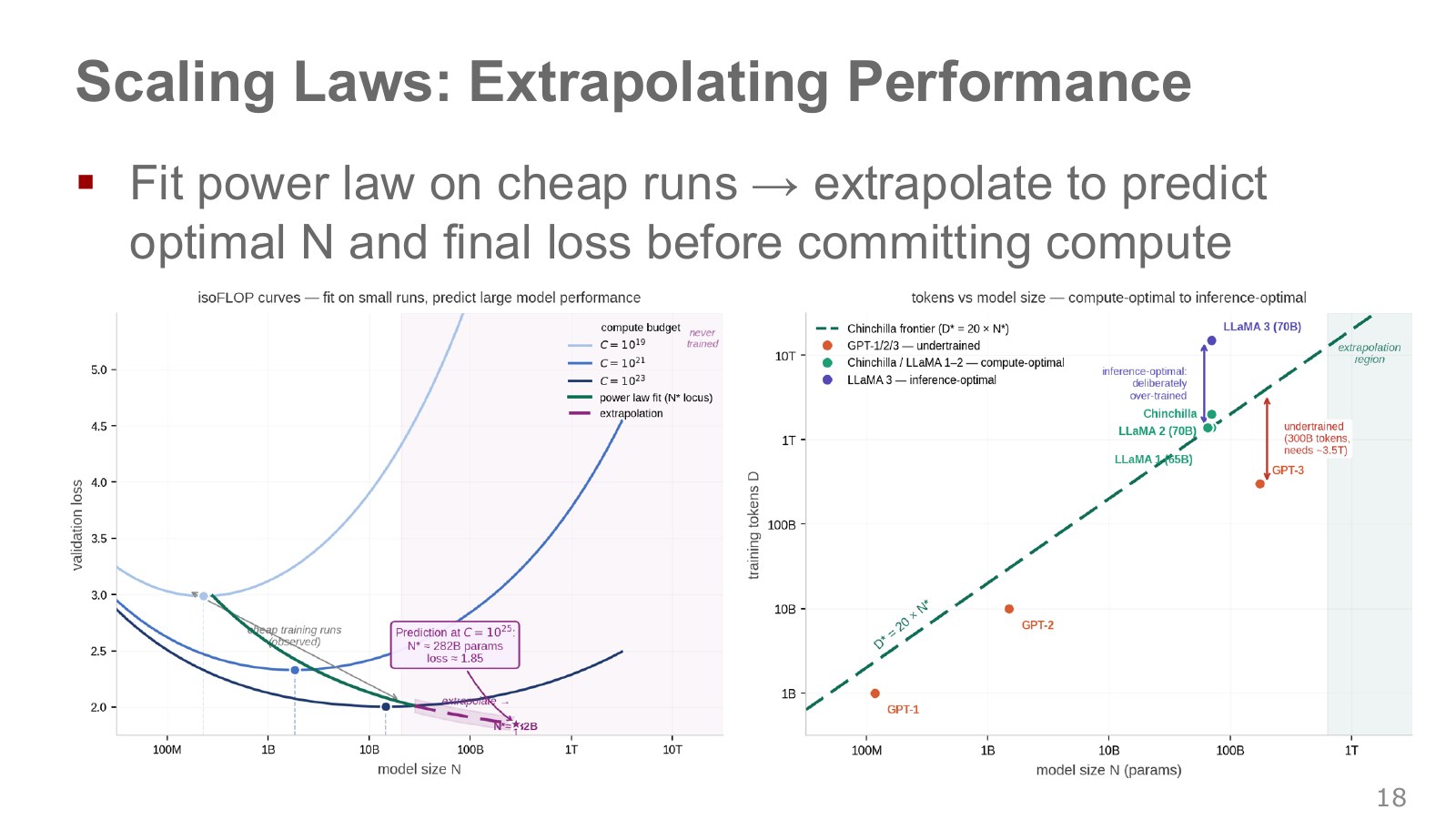
The isoflop curves on the left vary model size under equal compute budgets. Estimating minimum-loss positions across budgets can suggest favorable sizes for larger runs. Extrapolation predicts beyond observed ranges and therefore carries assumptions that the relationship continues, as well as uncertainty.
The model minimizing one training run’s cost may differ in size from the model minimizing total cost across many calls. Training a smaller model on more tokens can reduce per-call computation even if training lasts longer. Read Chinchilla’s token ratio as a budget-allocation result for that experiment. Chinchilla paper
The right side compares model sizes and training-token counts. Minimizing training computation alone differs from minimizing total cost over many deployed queries. A smaller model trained longer on more data can cost more initially while being cheaper to run repeatedly.
It is therefore unjustified to call training beyond 20 tokens per parameter an inherently wrong choice. Robot applications also depend on latency, power, device memory, and failure cost. Accurately extrapolating language-prediction loss does not imply equally accurate predictions of physical-task success or safety constraints.
#P020 · Turning visual information into Transformer input units
A robot must see the cup and hand positions as well as read instructions. Earlier embeddings converted words into numerical vectors. Next, we represent information from different image locations as vector units too.
A shared vector-sequence interface permits the same attention operations. But identical interfaces alone do not place language and images in a shared semantic space. First we examine image tokenization, then learning that connects meanings across the two data types.
#P021 · Image patches are pixel vectors, not words cut into numbered pieces
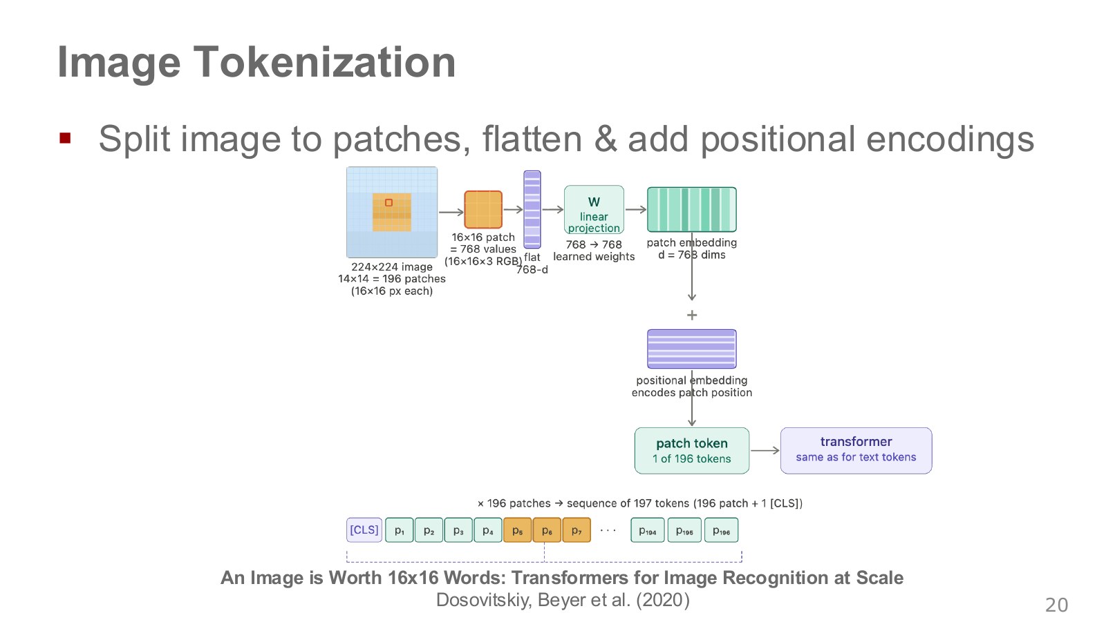
Dividing a 224×224 image into patches 16 pixels on each side gives 14×14=196 patches. Here, 16×16 is the patch’s pixel size, not a division into sixteen pieces along each image axis. One RGB patch flattens into 16×16×3=768 numbers.
A learned linear transformation maps that vector to the model dimension, then position information is added. The figure’s 768→768 is a dimensional choice for that example, not a requirement for every model. Position information distinguishes patches from the image’s top and bottom.
Including the special CLS classification token yields a sequence length of 197 in this example. Not every visual model uses CLS or passes only that single vector to other models. Later VLMs can pass multiple patch features into a language model. Vision Transformer paper.
#P022 · Matching dimensions is different from connecting meanings
Suppose apple-image patches and the word apple are represented by vectors of the same dimension. Equal length alone does not tell the model they have related meanings. Paired data and a learning objective are needed.
Here, alignment means learning corresponding representations across data types. Bringing whole-image and caption meanings together, answering questions using image information, and linking a particular word to an image location are different levels of alignment. CLIP’s strength at the first does not automatically provide precise object localization at the last.
#P023 · CLIP learns to retrieve matching image–text pairs
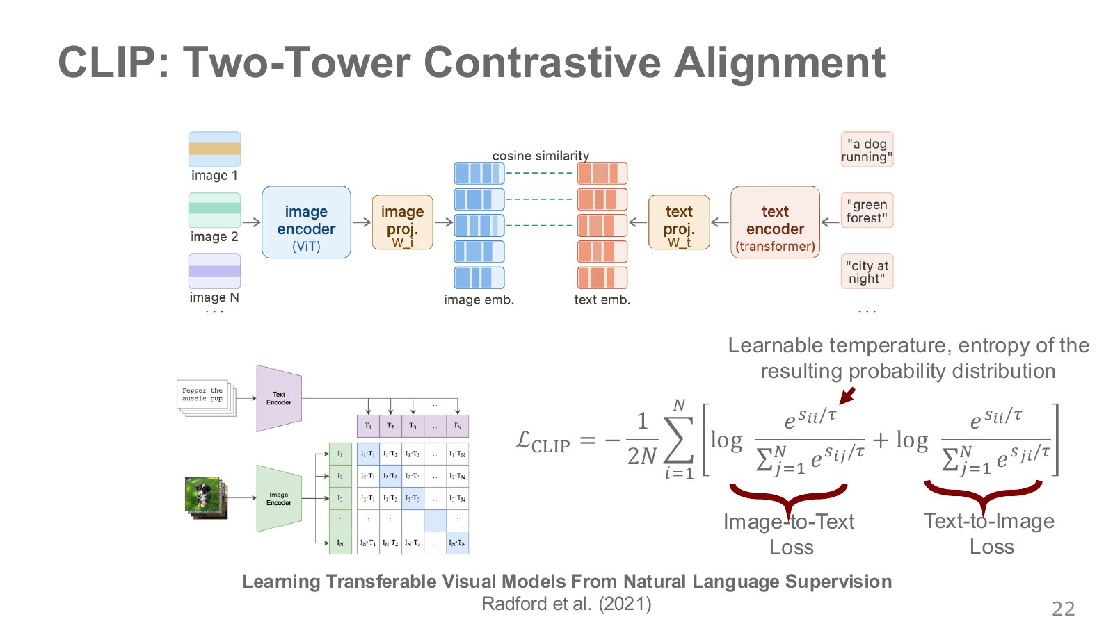
The two towers are image and text encoders. A batch of paired images and texts becomes vectors. Dot products of length-normalized vectors give cosine similarities in an × table. Matching row and column indices mark original pairs; training encourages each image to score its own text above the others. The reverse direction is trained too.
Explore the symbols and calculation A relative score for image selecting text within the batch
Read the equation in words
Normalize relative scores for one image's match among batch texts. Even for the same image, probabilities depend on the candidate set.
Understand each symbol
- The similarity score between image and text .
- A positive temperature making the distribution sharper or flatter, distinct from trajectory notation.
- The batch candidate count and relative probability of image selecting text .
- Add every term over the indicated range, computing one term and repeating through the end of the range.
- Conditional notation: the information to the right of the bar is given. This is not a division sign.
Follow the calculation
- Divide similarities between the image and all texts by a positive temperature.
- Exponentiate each score and divide by the sum across candidates.
Check with a small example
Candidate scores [0,1] at temperature 1 give probability approximately 0.731 for the second candidate. This is not the probability that an object exists in the image.
An illustrative example for understanding the equation.
Explore the symbols and calculation The bidirectional matching-pair loss
Read the equation in words
Train both image-to-text and text-to-image retrieval. Each direction reduces negative log probability of the correct match.
Understand each symbol
- The number of correct image–text pairs in one batch.
- The two normalized distributions selecting text from images and images from text.
- Matching indices indicate a correct pair.
- Add every term over the indicated range, computing one term and repeating through the end of the range.
- The natural logarithm. It converts products into sums and is defined only for positive inputs.
- Conditional notation: the information to the right of the bar is given. This is not a division sign.
Follow the calculation
- Calculate correct-pair probabilities in both directions.
- Negate and sum their logarithms, then divide by the number of directions and pairs.
Check with a small example
With two pairs and every correct-match probability equal to 0.5 in both directions, mean loss is approximately 0.693.
An illustrative example for understanding the equation.
Here, is similarity and a positive temperature. A lower temperature turns the same score differences into sharper selection probabilities. The reverse direction normalizes across images, rather than simply transposing the first probability table.
This structure alone does not make CLIP a language model generating sentences token by token. Multiple captions may correctly describe one image, so other batch pairs are not necessarily entirely wrong semantically. The original CLIP paper studies transferable visual representations learned by contrastive training. The figure depicts a ViT encoder example; the original paper also includes other image-encoder families.
#P024 · LLaVA inserts visual features into a sequence the language model can read
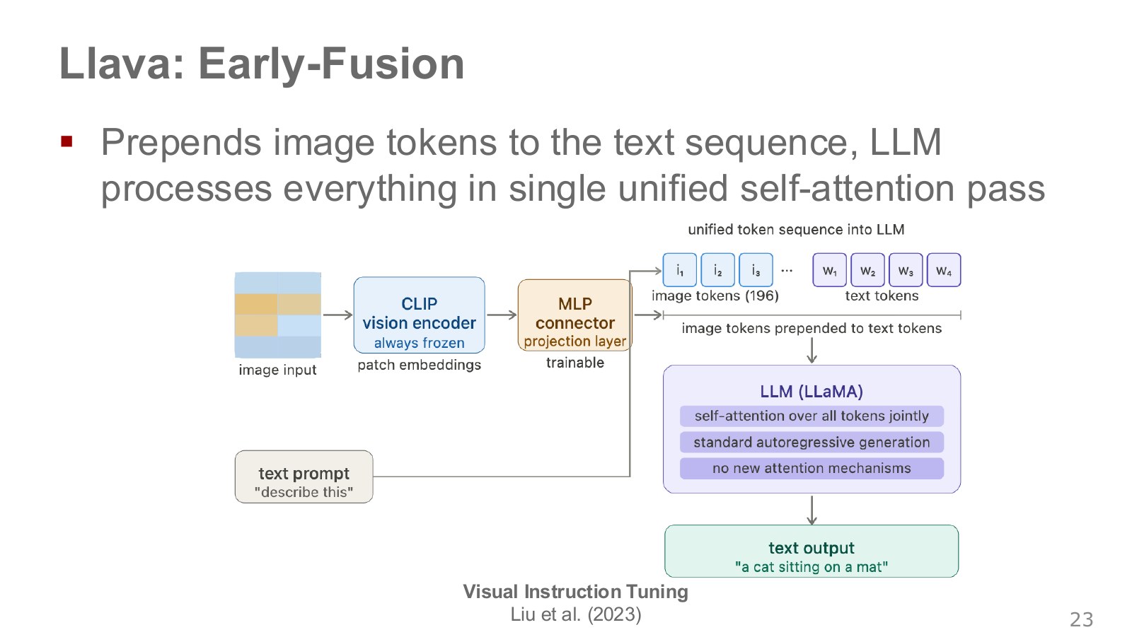
The image on the left passes through a visual encoder to produce multiple patch features. The connector maps their dimensions into the language model’s input space. These visual features then enter alongside text embeddings, letting attention reference both. The output answers a question such as “What is visible?” in words.
Here, early fusion means that image and text information enter shared sequence processing in the language model. It does not mean raw pixels and characters are handled identically. A visual encoder precedes them, and visual-feature format and count vary by version.
Distinguish linear projection in the original LLaVA paper from MLP connectors in later versions. Do not memorize the slide’s MLP as a universal LLaVA architecture. Frozen and trainable weights likewise vary by training stage and variant. Feature alignment and visual instruction tuning shift the objective from comparing image–text similarity to generating answers about images.
#P025 · Flamingo adds paths for language to reference visual information
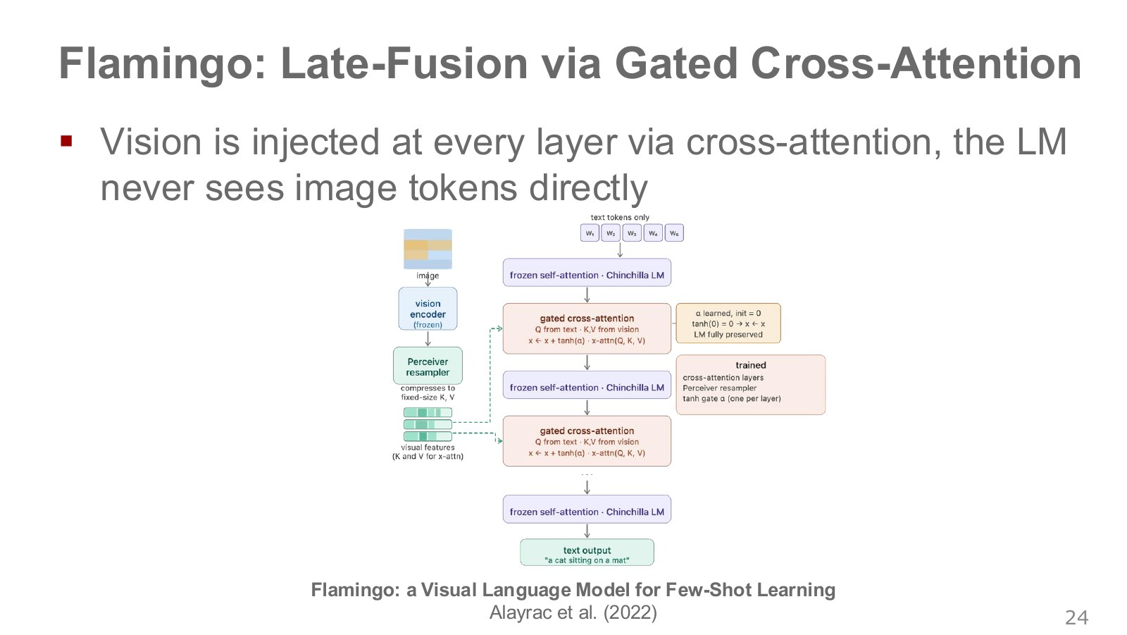
Visual-encoder features pass through a Perceiver Resampler into a fixed number of visual representations. Added gated cross-attention uses text queries to reference visual keys and values. This differs in where information meets from concatenating image and text tokens directly into one self-attention sequence.
Explore the symbols and calculation A conceptual gate controlling the addition of visual information
Read the equation in words
A gate controls how much visual information is added to language representations. An initial zero gate preserves the old representation despite adding the new visual pathway.
Understand each symbol
- Language hidden representations before and after combination. Here, is not an upper bound.
- A representation summarizing visual input.
- A learnable gate and its transformed value between −1 and 1.
- Cross-attention using language queries to reference visual keys and values.
Follow the calculation
- Use the language representation as a query to reference visual representations.
- Multiply the result by the gate value and add it to the existing language representation.
Check with a small example
Existing value 2, visual-path output 3, and transformed gate 0.5 give new value 3.5. At gate weight zero, the added contribution is zero.
An illustrative example for understanding the equation.
Initializing gate weight at zero makes the added path contribute nothing initially. Learning can then adjust its visual contribution. An important design feature is keeping pretrained language-model weights fixed while introducing this new pathway.
A gate opening over training describes a possible behavior, not a guaranteed monotonic increase. New-block spacing also depends on the configuration; it is not necessarily one in every layer of every model. Saying that the language model does not see image tokens directly means they are not appended to the same input sequence, not that visual information cannot affect the output. Original Flamingo paper.
#P026 · Joint multimodal learning still requires input formats and temporal alignment
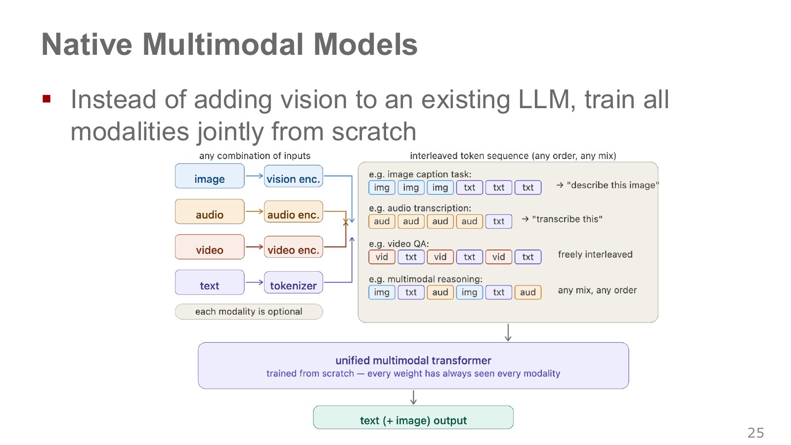
Images, audio, video, and text pass through their respective encoders or tokenizers. Examples on the right interleave units such as an image followed by a caption, audio followed by text, or video followed by a question. A common sequence model learns relationships across data types.
Native multimodal usually refers to training that tightly integrates multiple data types. The name alone does not prove every component was trained from random initialization or every weight saw each data type equally. Actual models may contain separate encoders, multiple training stages, different losses, and masks.
Combining audio and video with different time axes also requires timestamps and alignment. Matching vector dimensions alone does not identify simultaneous sounds and movements. The figure illustrates a joint-learning direction rather than detailed product specifications.
#P027 · Compare visual-information pathways rather than model names
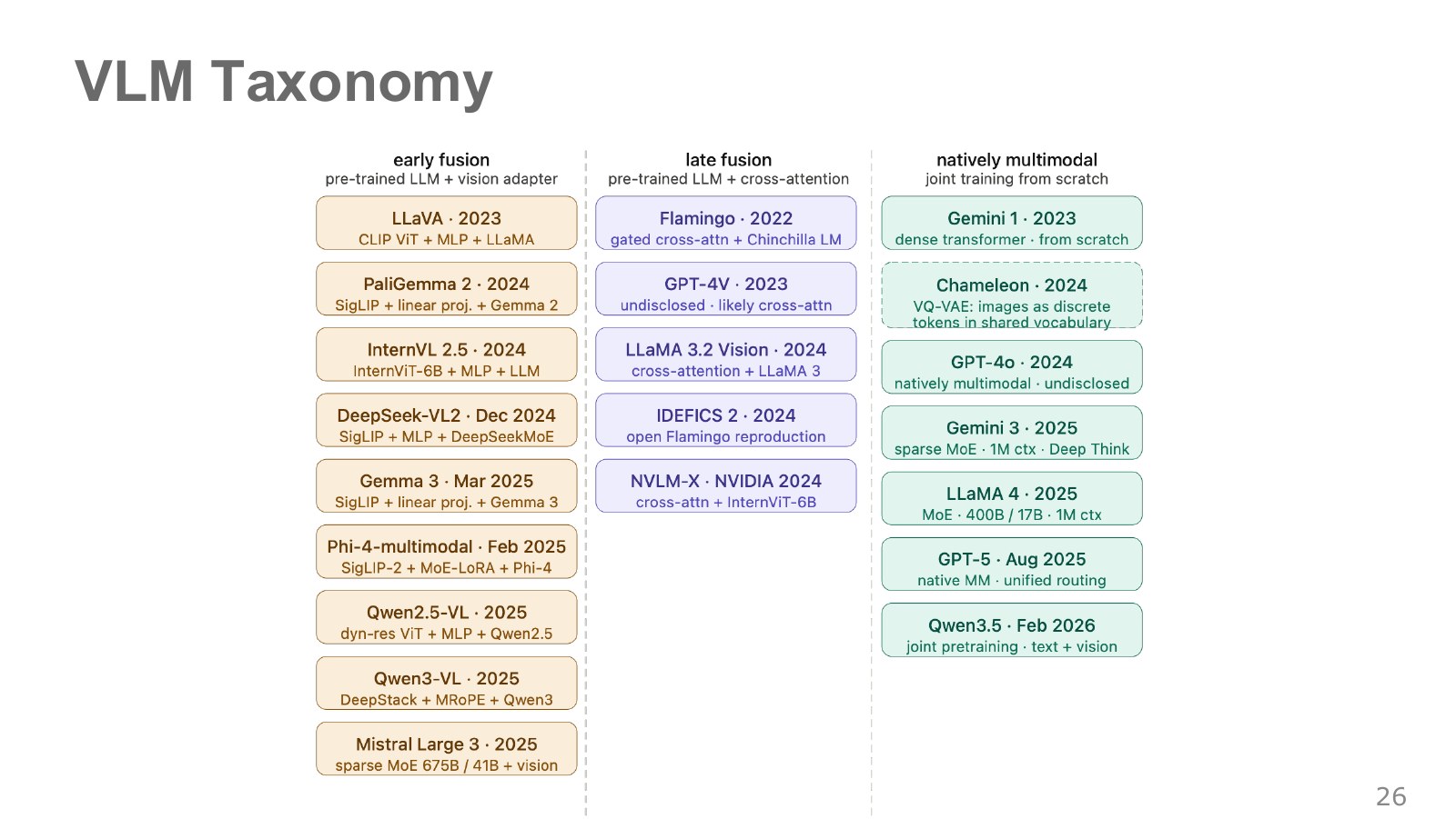
The three columns broadly contrast merging visual features into language sequences, adding separate cross-attention paths, and jointly training multiple data types. Reading the connector, added attention, and joint-learning differences first provides comparison criteria that remain useful as model names change.
The table mixes models with publicly documented architectures and models whose internals are insufficiently disclosed. Labels such as “likely” and “undisclosed” denote inference or missing disclosure. They should not be rewritten as verified architectural facts. An individual model may also combine characteristics from several columns.
This is not a quality ranking. Compare trainable-weight counts, visual-token counts, data, preservation of language capabilities, video length, and compute costs together. A model’s placement in one column does not mean it can produce robot joint commands.
#P028 · From seeing and answering to seeing and acting
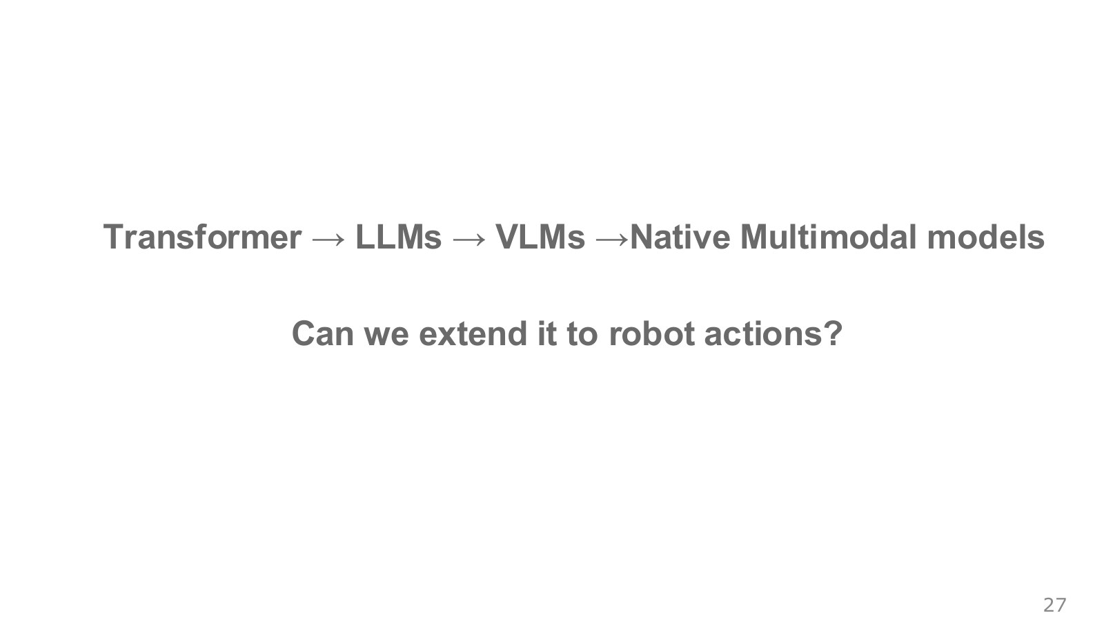
The question changes from “Where is the spoon?” to “Which commands will pick it up?” Image description ends with text output, but action output must connect to the actual robot’s kinematics, controller, and environment.
Actions can become model units just as language and images become tokens. But continuous-value resolution, different joint units, generation latency, and temporal consistency introduce new challenges. Action representations and execution interfaces matter alongside Transformer architecture.
#P029 · Action tokens become commands through a defined control interface
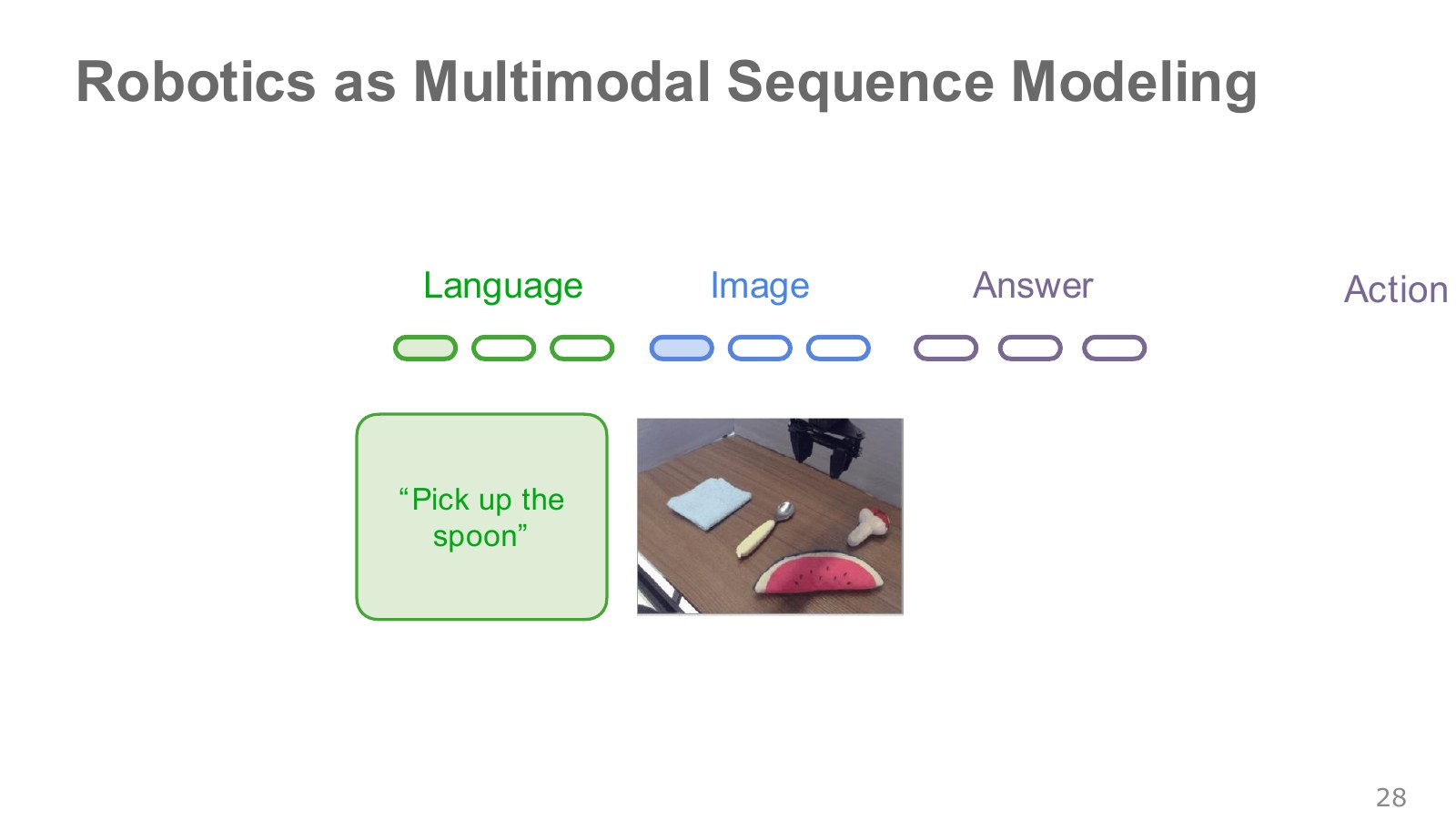
“Pick up the spoon” on the left supplies a language condition, while the central image shows the current scene. If the output represents actions instead of descriptive text, this forms a vision–language–action (VLA) model. Actions can encode hand displacement, rotational changes, and gripper opening.
An agreed decoder converts output tokens into numerical commands. The downstream control process differs depending on whether these numbers denote joint targets, relative end-effector positions, or velocities. Token indices are not sent directly to motors. A low-level controller still tracks the targets.
Including past images and actions in the actual input sequence allows history conditioning. But not every VLA takes a long history simply because it uses a Transformer; some use only a few current images. Distinguish architectural possibilities from actual input design.
#P030 · What is lost by dividing continuous actions into 256 bins?
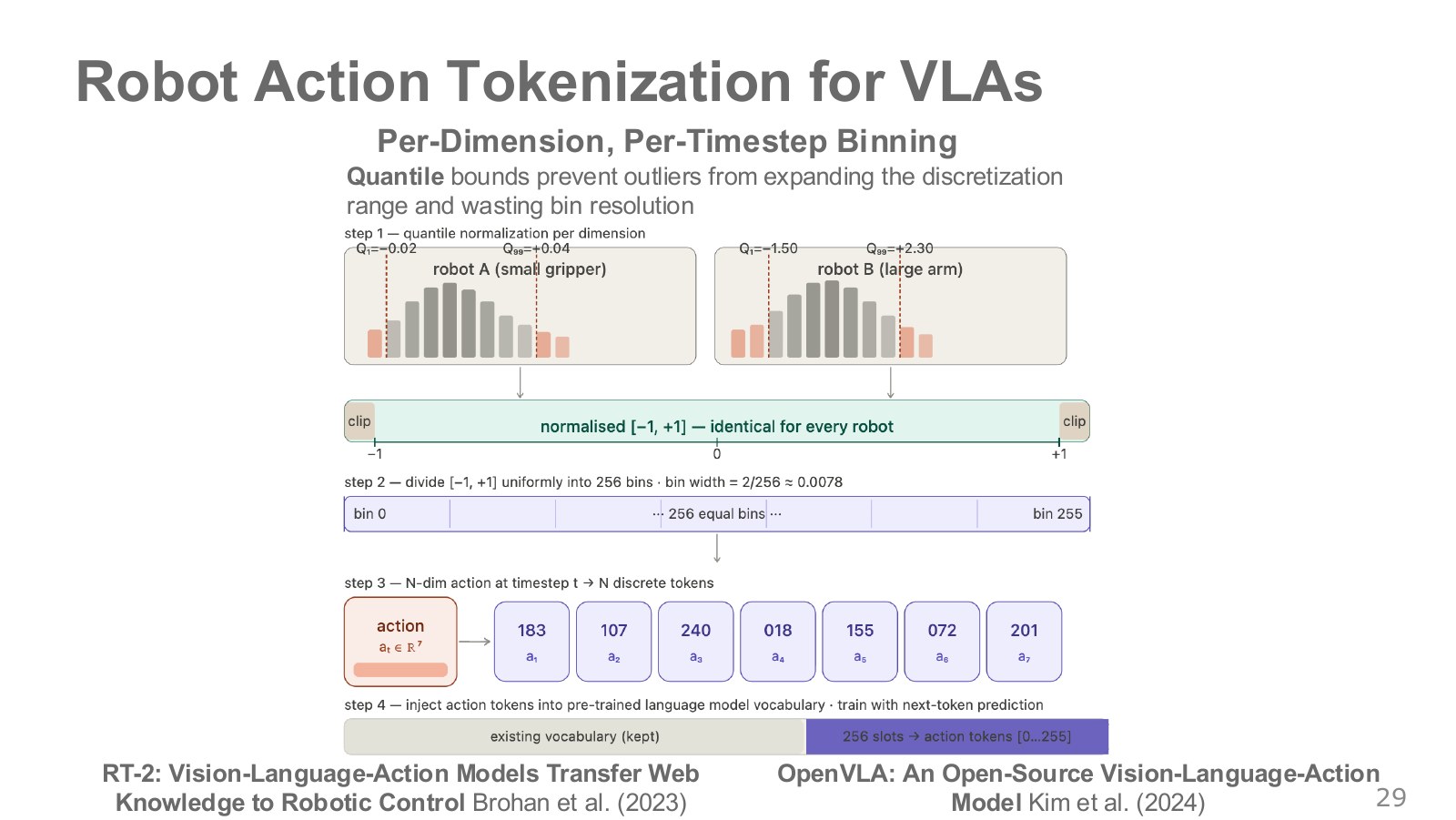
The histograms show two robots with different physical action ranges: small displacements on the left and a wider range on the right. Defining lower and upper quantiles for each action dimension and normalizing that range reduces the tendency of one rare extreme outlier to compress most values into a few narrow bins.
Explore the symbols and calculation Normalizing an action range to −1 through 1
Read the equation in words
Convert a physical action into a fraction between lower and upper reference values, then map it to −1 through 1. Training-data quantiles can provide these references.
Understand each symbol
- One component of the original action in physical units.
- Each component's distinct lower and upper reference values. Here, is not RNN memory.
- The normalized action between −1 and 1, distinct from control torque or an RNN memory vector.
- Clip an intermediate fraction below zero to zero and above one to one.
Follow the calculation
- Subtract the lower reference from the action and divide by the full reference range.
- Clip outside 0–1, multiply by 2, and subtract 1.
Check with a small example
For action references 0–10, original action 7.5 normalizes to 0.5. Original action 12 clips at the upper limit and becomes 1.
An illustrative example for understanding the equation.
Explore the symbols and calculation An example mapping normalized actions to bin indices 0–255
Read the equation in words
Convert a normalized continuous action into an integer identifying one of 256 bins. Grouping continuous values into bins loses some detail.
Understand each symbol
- The normalized action from the preceding equation.
- The action-bin index from 0 through 255.
- The floor function, returning the greatest integer no larger than the input.
- A safeguard preventing the endpoint from exceeding the last valid index.
Follow the calculation
- Map −1–1 to 0–1 and multiply by 256.
- Discard the fractional part; if the endpoint produces 256, restrict it to 255.
Check with a small example
Normalized −1 maps to index 0, 0 to 128, and 1 to 255 after restriction.
An illustrative example for understanding the equation.
The selected lower and upper quantiles and must differ. If is exactly 1, the calculation produces 256, so clip the last index to 255. Decoding with bin centers bounds in-range error by half a bin width in original units. Clipping errors outside the range do not share this bound.
The OpenVLA paper divides each dimension’s first-to-99th-percentile range into 256 bins. Distinguish this choice from the original RT-2 min–max method. Action tokens can be mapped into a language-model vocabulary; OpenVLA reuses some existing vocabulary slots.
Identical normalized indices do not mean identical physical motions across robots. Joint order, coordinate frames, absolute values versus increments, movement units, and gripper semantics must be aligned. Encoding each dimension of a seven-dimensional action with one index requires seven tokens per control instant.
#P031 · Action chunking and temporal ensembling address different problems
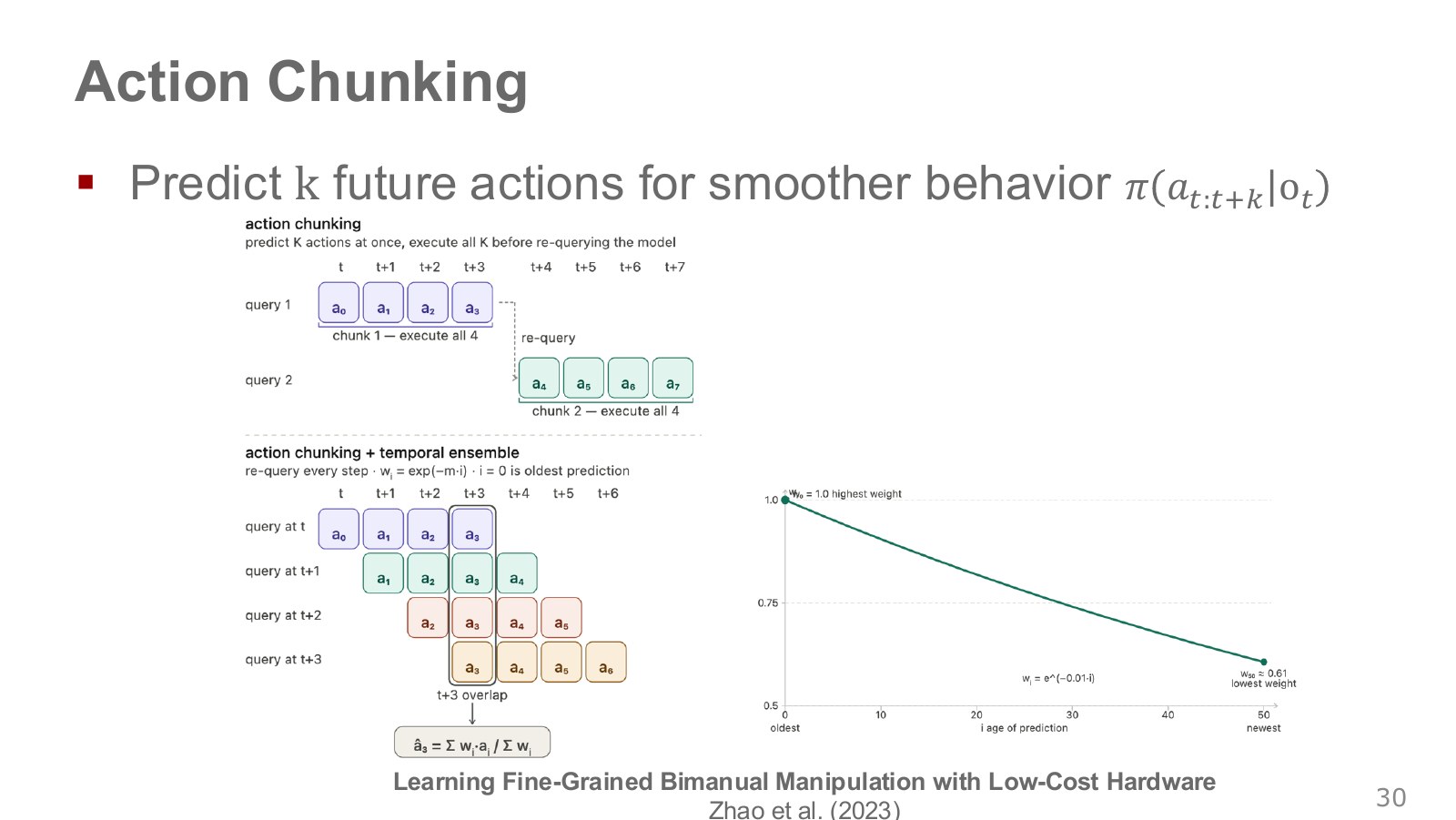
The upper timeline executes all four predicted actions before observing again. Actions within the chunk can be planned together, but observations are incorporated less frequently. The lower timeline predicts a fresh chunk every instant and combines predictions referring to the same actual execution time: earlier predictions of the present action are combined with the latest prediction of that same action.
Explore the symbols and calculation Combining overlapping predictions for the same execution time
Read the equation in words
Form a weighted average of actions predicted at different times for the same execution instant, smoothing boundaries across overlapping chunks.
Understand each symbol
- The action predicted for time by overlapping prediction .
- That prediction's weight and the number of overlapping predictions.
- The weighted-average action actually used.
- Add every term over the indicated range, computing one term and repeating through the end of the range.
Follow the calculation
- Collect only predictions corresponding to the current execution time.
- Sum weighted predictions and divide by the weight sum. The sum of positive weights must be nonzero.
Check with a small example
Predictions 1 and 3 weighted by 2 and 1 give executed action . The original ACT paper indexes exponential weights from the oldest prediction.
An illustrative example for understanding the equation.
The original ACT paper indexes the oldest prediction with =0 and uses exponentially decreasing weights. Under this notation, a positive decay coefficient therefore gives older predictions greater weight. Check the indices: this is opposite to the common assumption that the newest prediction receives the most weight. Our example verifies the distinction with predictions 1, 2, and 3 ordered oldest first.
This differs from a filter simply averaging actual actions across different times. It combines what overlapping plans say to do at the same time. It trades smoothness against responsiveness to new observations; if plans choose entirely different valid routes, their average need not be safe. Calling the policy at every instant also incurs computation.
#P032 · ACT does not generate 100 actions through 100 next-token steps
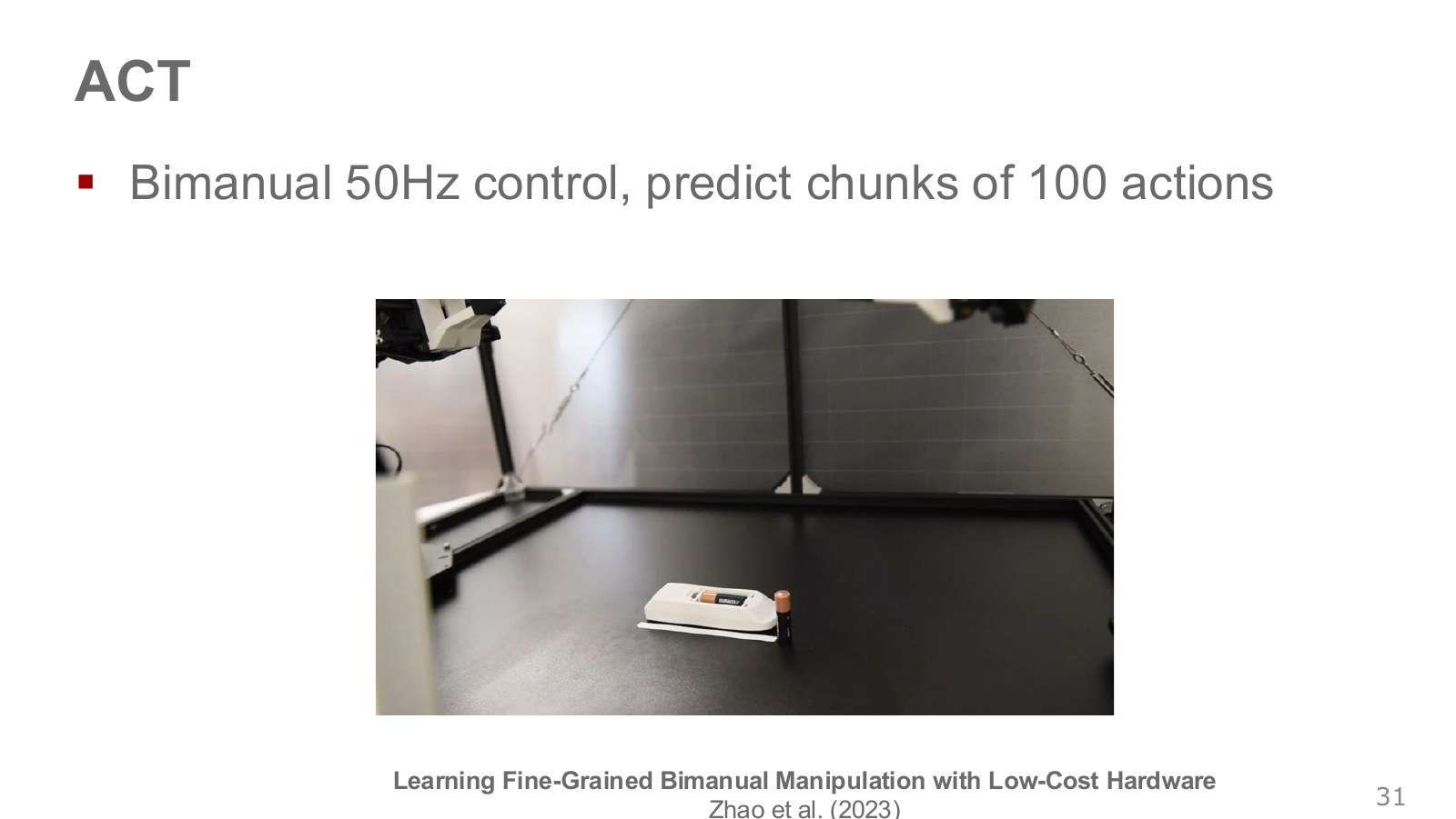
The battery-insertion video requires precise coordination of both hands and their contacts. ACT’s ALOHA setup controls a combined 14-dimensional action at 50 Hz and predicts chunks of length 100. One chunk spans about two seconds and contains 1,400 scalar values. It does not generate these 1,400 values one by one like language tokens.
The original paper combines a conditional VAE and Transformer. During training, an encoder uses demonstrated action chunks and joint states to infer a latent style distribution. The policy decoder predicts chunks from images, joint states, and style. This connects to Chapter 06’s latent-variable models.
At execution, future demonstrated actions are unavailable, so the training encoder is discarded. The original paper fixes style at zero, the prior mean, for deterministic decoding. It would therefore be inaccurate to describe ACT as an autoregressive VLA randomly sampling latent codes each time. Its flexible movements result from model, data, hardware, and control settings together; action chunking alone does not guarantee the same precision. Official project and code.
#P033 · Copying similar tokens can give low loss yet fail at fast control
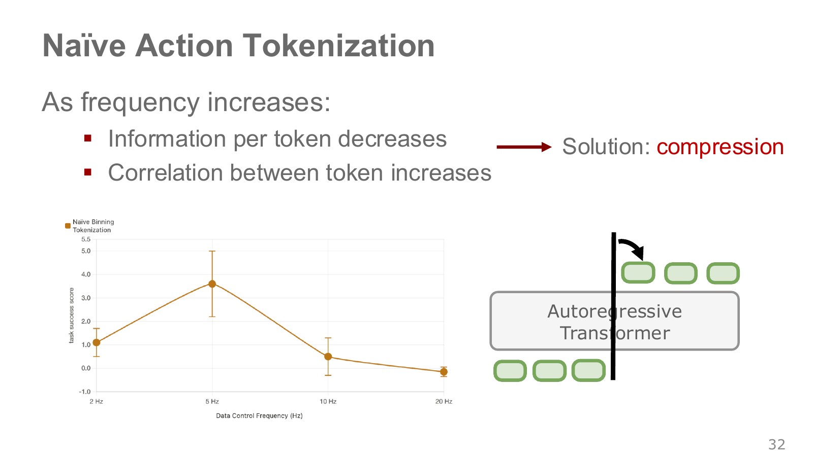
The left graph shows a simple binned-token policy deteriorating at higher data control frequencies in this experiment. The right emphasizes an autoregressive structure’s temptation to copy preceding tokens when neighboring actions are very similar. Recording physically continuous motion at short intervals creates nearly identical adjacent values.
At higher control frequencies, neighboring joint commands differ less. A model copying the previous token can appear strong during training yet miss small necessary changes, such as when a battery contacts its slot. FAST compresses temporal structure across action chunks rather than isolated instants. FAST project
Teacher forcing supplies the actual preceding action, so predicting a nearly identical next value can achieve high token accuracy. But repeatedly feeding back predictions at execution can suppress necessary changes or accumulate errors. This is why token accuracy and long-task success should be checked separately.
High control frequency means more commands per second, not necessarily rapidly oscillating action signals. Sampling the same smooth curve more frequently increases both sample count and redundancy. Do not generalize this experiment into a limitation of every high-frequency controller or Transformer.
#P034 · Transform temporal motion into frequency coefficients with DCT, then compress
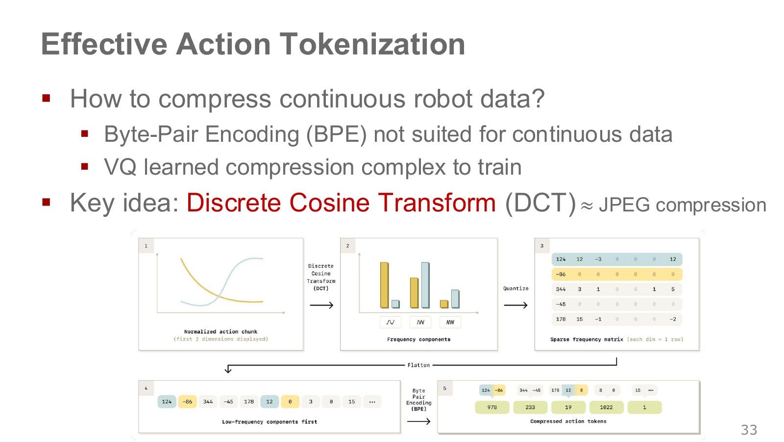
Read the five boxes in order. First, normalize action sequences per dimension. Second, apply the discrete cosine transform (DCT) to each dimension’s temporal signal, expressing broad trends and fast changes as coefficients of different cosine components. Third, scale and round coefficients to integers. Fourth, flatten dimensions starting with low frequencies. Fifth, apply BPE to repeated integer patterns to produce final tokens.
Explore the symbols and calculation An orthonormal DCT-II for one action dimension
Read the equation in words
Transform a temporal action signal into coefficients measuring similarity to cosine components. Smooth changes tend to concentrate in lower frequencies.
Understand each symbol
- The values over time for one action dimension and the chunk length.
- A frequency-component index and its coefficient.
- The orthonormal scaling coefficient balancing frequency magnitudes.
- Here, the circle constant pi, not an action policy.
- Add every term over the indicated range, computing one term and repeating through the end of the range.
Follow the calculation
- Multiply each action value by the corresponding frequency's cosine and sum across time.
- Apply the frequency-dependent normalization. Retaining all coefficients permits inversion.
Check with a small example
The length-two transform of constant actions [1,1] has first coefficient and the remaining coefficient zero, concentrating the average motion in the first coefficient.
An illustrative example for understanding the equation.
Explore the symbols and calculation Coefficient normalization and integer quantization
Read the equation in words
Balance the zero-frequency and other-frequency magnitudes, then scale real coefficients and round to integers. Rounding introduces reconstruction error.
Understand each symbol
- Normalization coefficients for frequency zero and other frequencies, and the action-chunk length.
- The scaling factor controlling integer resolution, not a reinforcement-learning discount factor.
- The real frequency coefficient and rounded integer symbol.
- Rounding to the nearest integer.
Follow the calculation
- Select the normalization coefficient for the frequency index.
- Scale the real DCT coefficient and round; divide by that scale during reconstruction.
Check with a small example
Coefficient 0.26 at scale 10 gives integer code 3 and reconstructed coefficient 0.3. Error 0.04 is within this scale's maximum rounding error 0.05.
An illustrative example for understanding the equation.
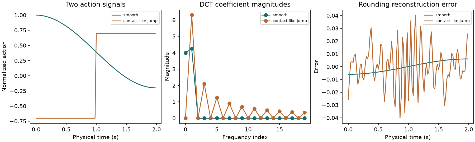
Here, is chunk length, the frequency-component index, and the scaling factor controlling rounding resolution. DCT itself is invertible if all coefficients are retained. Loss arises mainly from rounding and range limits. Small coefficients rounded to zero form long repeated patterns that BPE can encode compactly. BPE itself groups integer symbols reversibly.
Smooth motions tend to concentrate energy at low frequencies. But high-frequency components at contacts or abrupt transitions are not always unnecessary noise. Lowering for stronger compression can lose important fine motions. The connection is that BPE is difficult to apply directly to continuous values, yet becomes useful again after DCT and integer conversion. Original FAST paper.
#P035 · Check which computation a fivefold improvement compares
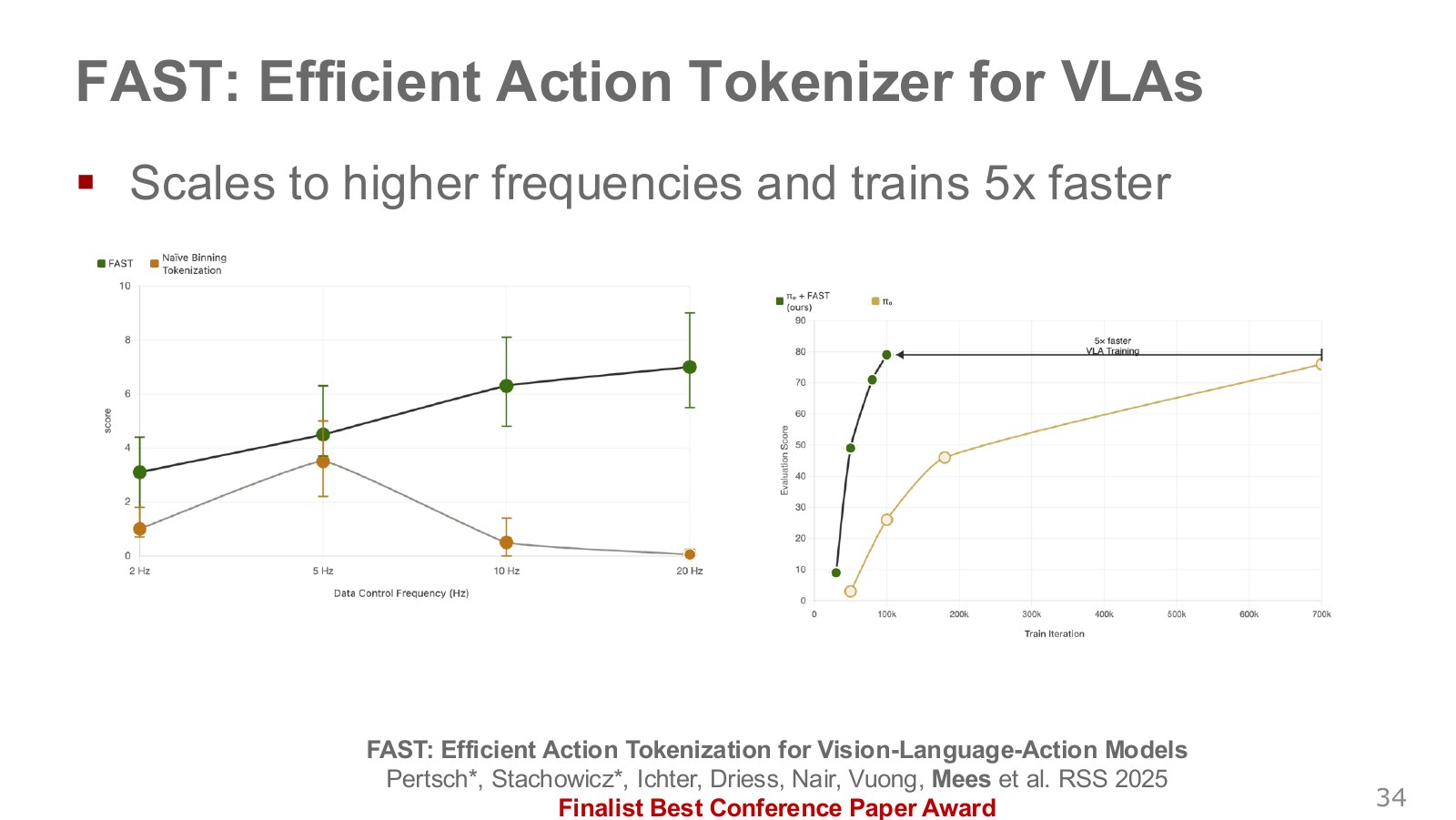
The left graph plots evaluation score against the data’s control frequency. In this setting, FAST tends to maintain or improve performance on high-frequency data compared with simple binning. Error bars represent variation across runs or evaluations; differences between mean points are not absolute laws.
The right graph plots training iterations against evaluation score. Although the lecture says “test time” at one point, the fivefold claim in this graph should not be read as fivefold lower generation latency. The paper reports improved training speed toward performance comparable with diffusion policies in the evaluated setting. This does not guarantee the same runtime improvement across every task, device, and model.
Autoregressive policies using FAST and Chapter 06’s flow-matching policies generate actions differently. Even with shared underlying vision–language representations, compare their output representations and training objectives separately. Official FAST research page.
#P036 · Generality and dexterity require different evaluations
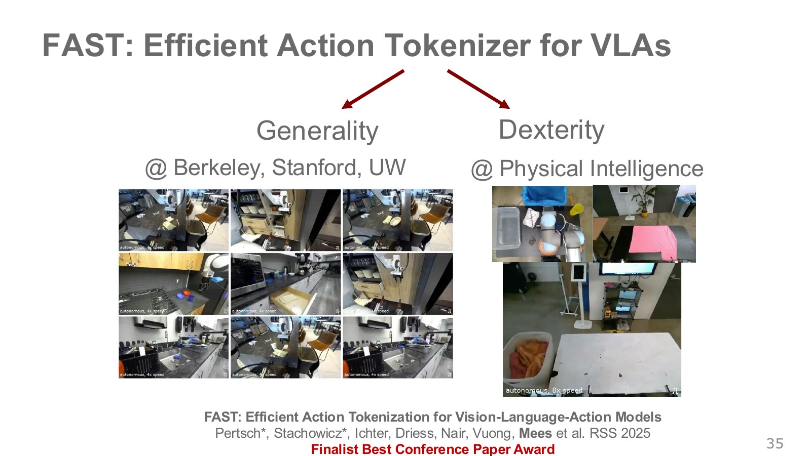
The photographs on the left show tasks across multiple kitchens and environments; those on the right show precise, long-horizon dual-arm tasks such as folding laundry. Generality concerns performance with new objects, scenes, and instructions; dexterity concerns reliable control and contact under tight error tolerances.
FAST experiments examine scaling in both directions. Evaluation in unseen kitchens does not imply unconditional operation on any robot or object. Check the data, hardware, instruction range, and success criteria together.
The publicly released general-purpose action tokenizer FAST+ provides a starting point for other datasets. Action dimensions, units, normalization, and lengths must still match, and downloading a tokenizer does not train a robot policy. Our examples are small calculations illustrating its principles, not reproductions of the photographed real-world tasks.
#P037 · Design what to remember and what to generate together
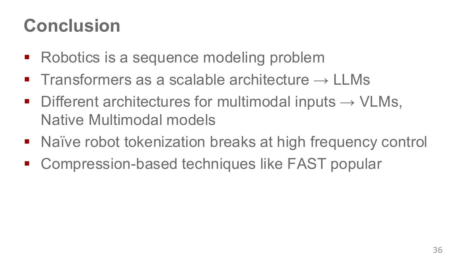
The chapter’s progression suggests three questions. First, is the current observation sufficient, or are past actions and observations needed? Second, should data be represented as characters, patches, continuous vectors, or action tokens? Third, does the model output autoregressive tokens, an action chunk in one pass, or actions iteratively updated through diffusion or flow?
| Method or concept | Problem addressed | What it does not guarantee by itself |
|---|---|---|
| History conditioning | Using past information absent from the current scene | Complete hidden-state reconstruction |
| Attention and position information | Learning contextual relations and order | Unlimited memory or constant total computation |
| CLIP and VLMs | Connecting visual and language representations and outputs | Precise position control or action success |
| ACT and action chunks | Jointly predicting actions across multiple times | Immediate response to every environmental change |
| FAST | Efficiently representing continuous actions as sequences | Lossless compression or safe execution |
Transformers provide structure for learning relationships between memory and action. Real-robot outcomes depend jointly on data, representations, objectives, generation latency, controllers, and evaluation. Look beyond token accuracy or language-model loss to whether the task finishes under real-time constraints.
#Further connection: Decision Transformer also takes the desired outcome as input
Decision Transformer, an official week-seven paper-discussion reading, connects sequence modeling with reinforcement learning. We discuss it as supplementary material rather than implying that the original lecture slides contain a separate algorithm section for it.
For each stored trajectory, calculate return-to-go—the sum of rewards from each time onward—and interleave these values with states and actions in a sequence.
Explore the symbols and calculation A trajectory representation containing return-to-go
Read the equation in words
Include the desired remaining reward alongside states and actions in the sequence. Decision Transformer uses this representation to predict actions conditioned on desired performance.
Understand each symbol
- The return collecting rewards after the current time. Check the sum to see whether discounting is used and where reward counting starts.
- The reward received at one step: a learning signal defined so that larger is better.
- The length of a trajectory or sequence. Here it sets how many steps enter the sum or product.
- Add every term over the indicated range, computing one term and repeating through the end of the range.
Follow the calculation
- Sum rewards from each time step to the end of a training trajectory.
- Interleave remaining return, state, and action; at execution, predict actions conditioned on a target return.
Check with a small example
Rewards [1,2,3] give remaining returns [6,5,3]. Receiving reward 1 from an execution target of 6 can reduce the remaining target to 5. A large target does not guarantee performance beyond the data.
An illustrative example for understanding the equation.
Training uses returns calculated from observed trajectories. Execution conditions action prediction on a desired return, current state, and history. Received rewards reduce the remaining target return accordingly. This is an offline RL approach distinct from repeatedly updating values through Bellman equations or directly calculating policy gradients.
Writing a large desired return does not ensure it can be achieved. Requesting actions and outcomes unsupported by training data creates extrapolation problems. Conditioning on context examples also does not make this equivalent to using prompts without training: model weights must first be learned from trajectories. Continuous actions can use a continuous-action prediction loss, as in the original paper, so outputs need not all be integer tokens from a language vocabulary.
#Executed examples and further reading
The example code and numerical results cover attention weights, future masking, input permutation, teacher-forcing loss, small character-BPE round trips, quantile-binning boundaries and error, ACT temporal ensembling, and DCT quantization and reconstruction. They also check that changing future target tokens leaves earlier outputs unchanged. These calculations do not constitute neural-policy training, real-robot execution, or physics simulation.
- Official Stanford CS25 recording: Andrej Karpathy’s explanation at 23:38–28:12 connects to , , , and multiple heads.
- Stanford CS224n 2024 Transformer slides: supplementary material on attention, position information, and the original encoder–decoder architecture.
- NTU 2021 self-attention lecture: the public English captions at 24:57–30:03 explain score calculation and weighted value sums. The original PPTX and PDF are also preserved in the source archive.
- Attention Is All You Need: the foundations of scaled dot-product attention, training, and parallelism.
- ACT and ALOHA project: the original paper, code, and physical-manipulation videos. Distinguish them from our own examples.
- Official FAST project: action-token compression and public tokenizer resources. The article’s DCT example does not substitute for running that released model.
- Humanoid Locomotion as Next Token Prediction: another example from the official discussion list. The article does not reproduce its full experiments.
Copyright in the slides and lecture belongs to Oier Mees and the rights holders of each cited resource. JJo created the explanatory text and numerical figures. Photographs, paper figures, and demonstration videos belong to their original authors. Oier Mees · ETH Computer Vision and Geometry Group.