Which way should an arm move just before grasping a cup? Looking only at whether the hand gets closer can miss the benefit of a temporary detour around a collision. Reinforcement learning evaluates consequences beyond the immediate action in one number, then uses that assessment to change behavior. This chapter asks how to calculate and learn that number: value.
Oier Mees · ETH Zurich 2026, Lecture 4 · Official course · Original PDF
#P001 · From predicting expert actions to finding good outcomes
Behavior cloning in Chapter 03 used the expert’s action in a situation as its target. Now we use rewards received after the robot acts to find a rule for better future outcomes. Reward is an evaluation signal, not an answer directly specifying a motor command.
We begin by listing every state in a small table and calculating values exactly. Next we learn values from observed transitions, and finally replace the table with a neural network to handle images and continuous actions. Distinguishing what is already known from what must be learned connects these three stages.
#P002 · Following demonstrations and earning more reward are different objectives
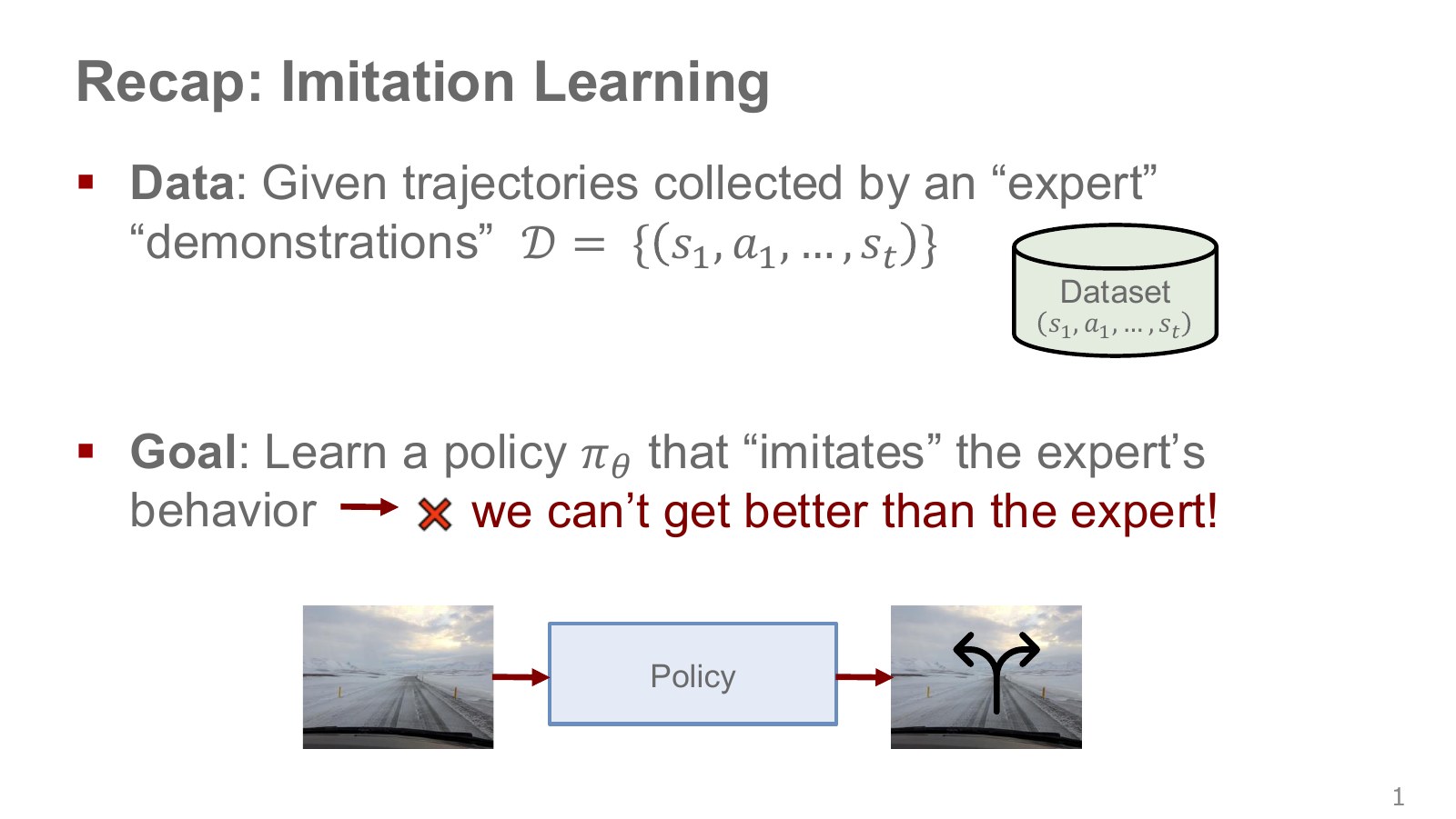
The dataset cylinder contains expert state–action trajectories. The road image passing through a policy box into steering illustrates training a model to map observations to demonstrated behavior.
The basic behavior-cloning loss does not require finding a higher cumulative reward than the expert. Matching a demonstration can remain the objective even when it is mistaken or slow. Reinforcement learning changes the evaluation criterion to cumulative reward, offering a way to improve beyond those limitations.
The figure’s statement that a learner “cannot outperform the expert” emphasizes this objective difference. It should not be read as a universal mathematical impossibility for every imitation learner on every evaluation. Generalization or combining demonstrations can change performance, but behavior cloning alone does not guarantee reward improvement.
#P003 · Bundling state, action, next state and reward into one experience
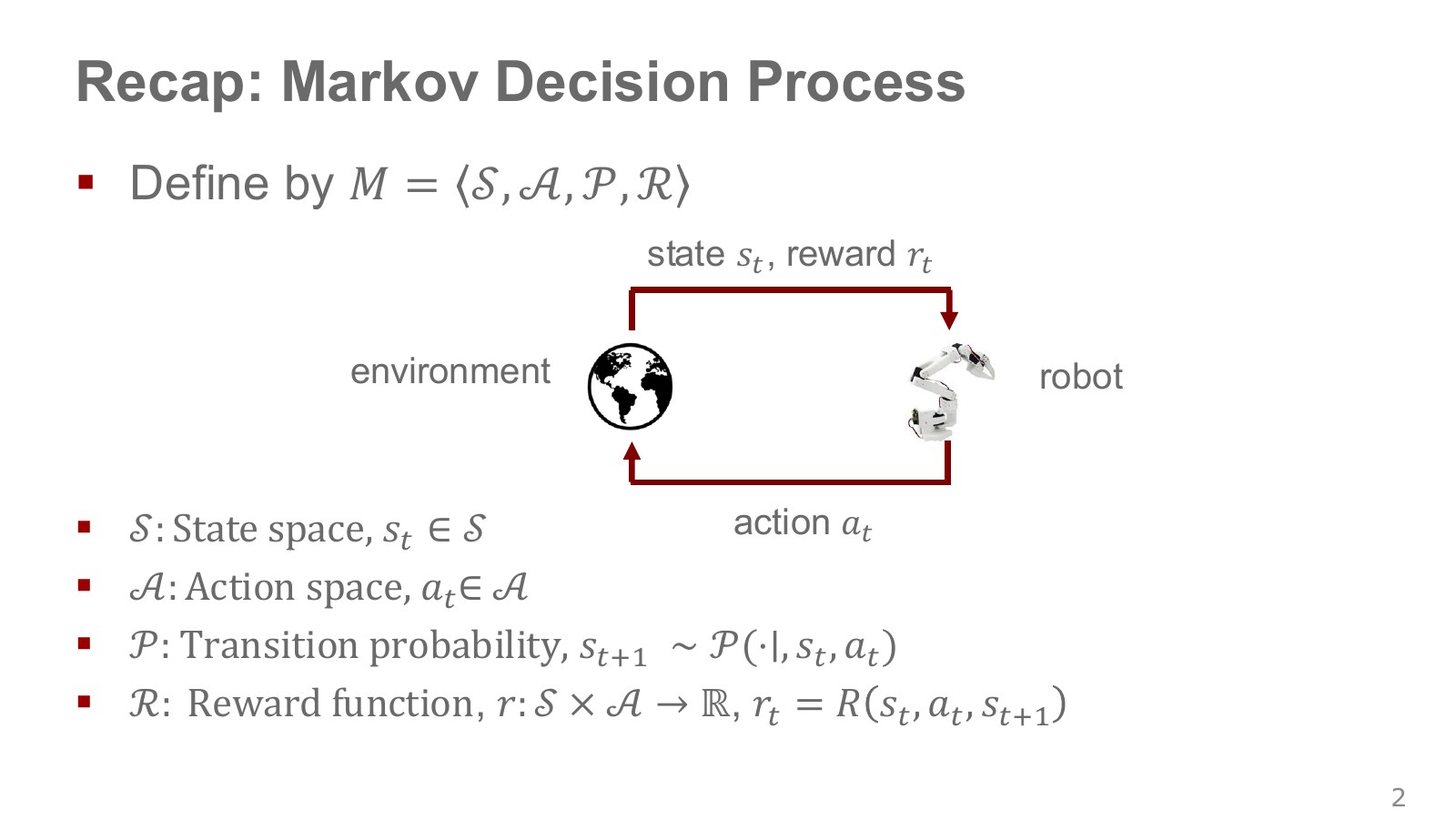
A Markov decision process (MDP) represents repeated agent–environment interaction. State space contains possible states, and action space possible commands. Transition specifies the likelihood of next state after action in current state .
The upper arrow carries state and reward back from the environment; the lower arrow carries the robot’s action into it. One execution step produces the following record.
Explore the symbols and calculation A transition records the current state, executed action, received reward, and next state
Read the equation in words
One moment of interaction with the environment is recorded as four items: the previous state, action, reward, and next state. This is one basic training example in reinforcement learning.
Understand each symbol
- The state at step , containing information such as position and velocity needed to predict what happens next.
- The action chosen at step : for example, a torque, a joint target or a movement direction, depending on the setup.
- The reward received at one step: a learning signal defined so that larger is better.
- The next state reached after executing the action.
Follow the calculation
- Store the state before acting and the selected action.
- Record the resulting reward and next state together with them.
Check with a small example
Being in front of a door, pushing it, receiving a success reward of 1, and reaching the open-door state constitute one transition.
An illustrative example for understanding the equation.
indexes physical execution, whereas below counts computational iterations. Reward may depend on the next state and is written . When an expression abbreviates it as , read it as the expected immediate reward for that state–action transition. The source also uses both reward-function conventions.
For cup grasping, state may include joint positions, velocities and object arrangements; actions may be tool-tip displacements or torques. With image observations alone, separately assess whether they constitute a full Markov state. Follow Chapter 02 for the state–observation distinction.
#P004 · Evaluating a sum over time, beyond one immediate reward
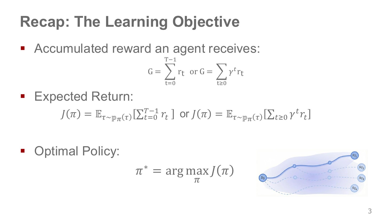
A return sums rewards from a rollout. Discount factor gives more distant rewards smaller weights. In the expression below, is the number of steps in a finite rollout.
Explore the symbols and calculation Policy performance is defined as the average discounted return over the trajectories the policy can generate
Read the equation in words
Within a trajectory, add the discounted rewards. Policy performance averages those trajectory returns under the policy.
Understand each symbol
- The return collecting rewards after the current time. Check the sum to see whether discounting is used and where reward counting starts.
- The reward received at one step: a learning signal defined so that larger is better.
- The discount factor for future rewards. Zero considers only the immediate reward, while values near one give more weight to the distant future.
- The length of a trajectory or sequence. Here it sets how many steps enter the sum or product.
- One trajectory containing states and actions in time order. This symbol does not denote an angle.
- A policy choosing actions given a state. A stochastic policy outputs probabilities or probability densities for actions.
- The policy's expected return.
- Add every term over the indicated range, computing one term and repeating through the end of the range.
- An expectation: an average over possible outcomes weighted by their probabilities.
Follow the calculation
- Multiply each reward by its time-dependent discount weight and add them.
- Average the possible trajectories according to their probabilities.
Check with a small example
If trajectories with return 2 occur 75% of the time and those with return 6 occur 25% of the time, policy performance is .
An illustrative example for understanding the equation.
is a time-ordered state–action trajectory, the policy, and an average weighted by possible outcomes’ probabilities. Like the branching paths on the right, one policy can produce different runs through disturbances or stochastic actions. One successful video does not establish expected performance.
An optimal policy maximizes expected return. While denotes the greatest value, denotes the choice attaining it. Multiple policies may tie. Infinite-horizon sums commonly use bounded rewards and .
#P005 · Why differentiating a step-shaped reward is difficult
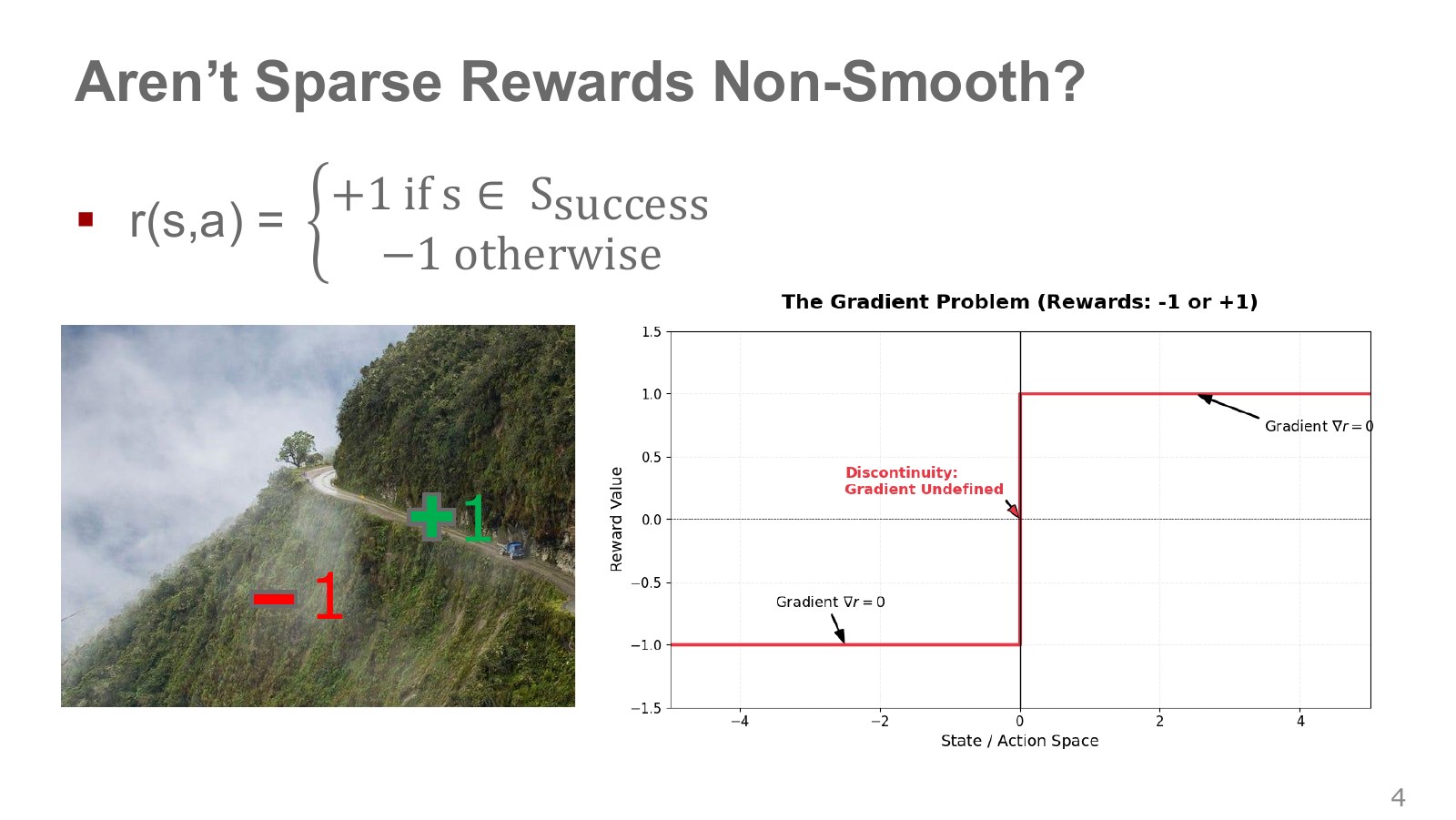
Consider a simple reward of +1 on the path and −1 beyond a cliff. The red line jumps between outcomes as a step function. On flat regions, a small position change leaves reward unchanged, giving derivative zero; at the boundary, an ordinary derivative is undefined.
A method that makes tiny changes to position or action and directly follows this reward’s gradient therefore obtains little useful direction for improvement. The boundary does not offer an enormous gradient that can simply be followed either.
Sparse and discontinuous rewards are different. Sparse means meaningful rewards arrive infrequently; discontinuous means a value jumps as its input changes. This example uses a binary outcome, but sparse rewards do not all have an identical step-function shape.
#P006 · A discrete outcome can still have a smoothly changing probability
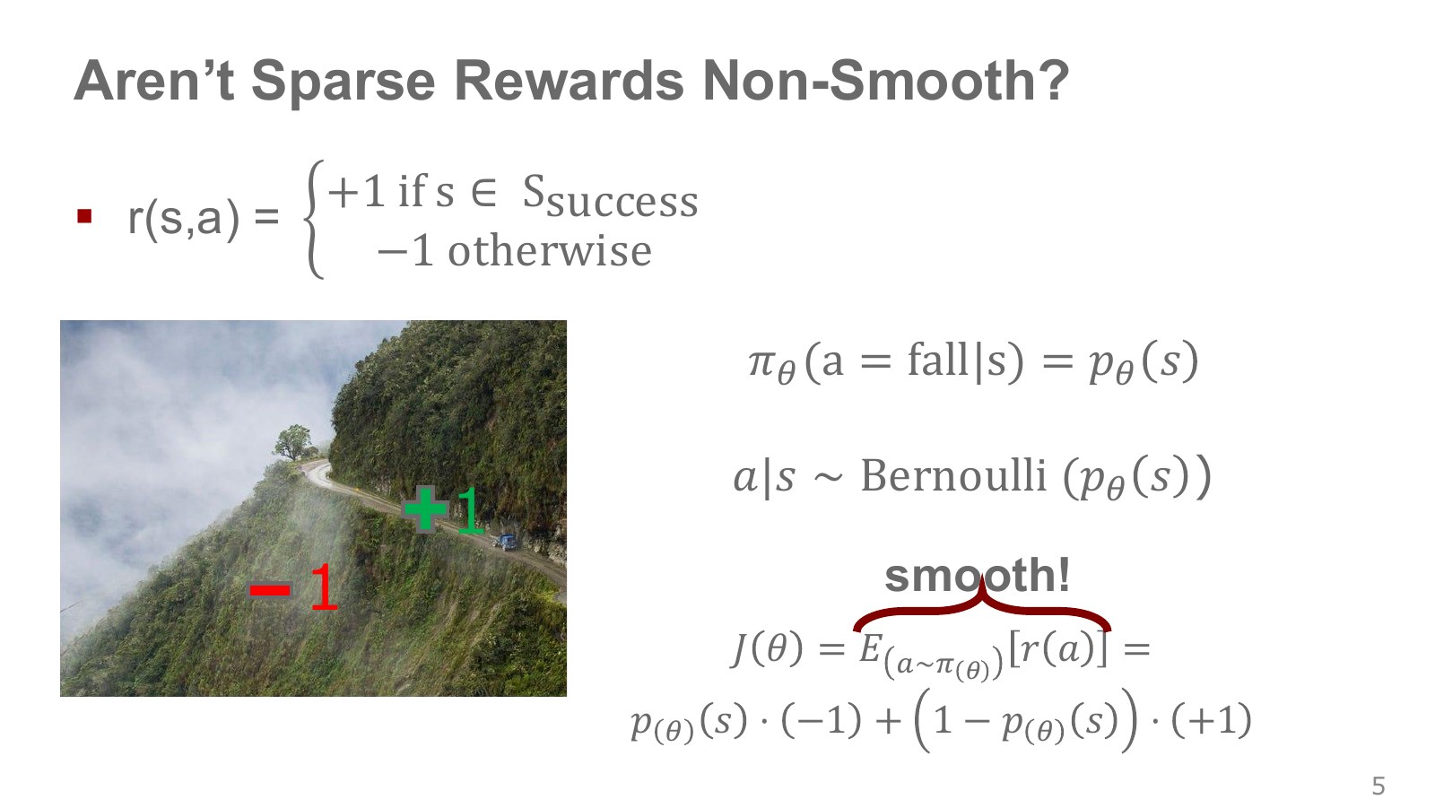
Let be the failure probability from the current state and the policy parameters. Modeling failure as a binary Bernoulli variable lets us calculate expected reward using failure and success probabilities.
Explore the symbols and calculation Reducing failure probability increases the expected binary reward
Read the equation in words
When failure gives −1 and success gives +1, expected reward can be written using failure probability alone. Reducing failure probability therefore increases expected reward.
Understand each symbol
- The parameters collecting the trainable weights of the network or policy.
- The probability that the policy fails from the state. In this example, is not a state-visitation distribution.
- The expected reward, which depends on the policy weights.
Follow the calculation
- Multiply the failure reward by failure probability and the success reward by success probability.
- Add the two terms and write success probability as one minus failure probability.
Check with a small example
With failure probability 0.2, expected reward is .
An illustrative example for understanding the equation.
A failure probability of 0.1 gives expected reward 0.8. It does not mean a single execution earns 0.8: each still receives +1 or −1, while many executions average to 0.8.
If failure probability is differentiable in the parameters, expected reward can be differentiated through it. Differentiating an outcome’s reward directly differs from changing the probability of a favorable outcome. Stochastic policies do not automatically make every objective smooth; distributional smoothness and conditions for interchanging expectation and differentiation matter.
#P007 · Read the red step and blue curve with attention to their horizontal axes
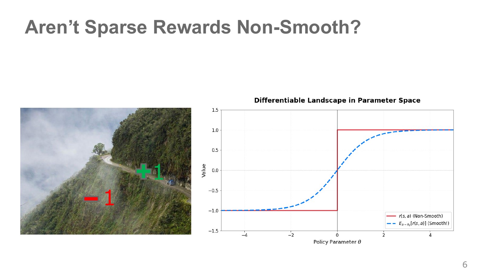
The red step describes whether a particular outcome is good or bad; the dashed blue curve describes average outcomes as the policy changes. The horizontal axis is policy parameters. An upward blue curve illustrates adjustments assigning more probability to success.
The preceding section defined as failure probability, so increasing it lowers expected reward. Before comparing it with the rising curve, check whether a symbol denotes success or failure. Do not treat the two source curves as interchangeable functions of the same input without their conditions.
This motivates how policy-gradient methods can learn even from binary rewards. Value iteration and Q-learning in this chapter instead use recursive value relationships and sampled updates, without differentiating reward directly. Reinforcement-learning algorithms do not all perform gradient descent on the blue curve.
#P008 · Predicting the remaining outcome before a rollout ends
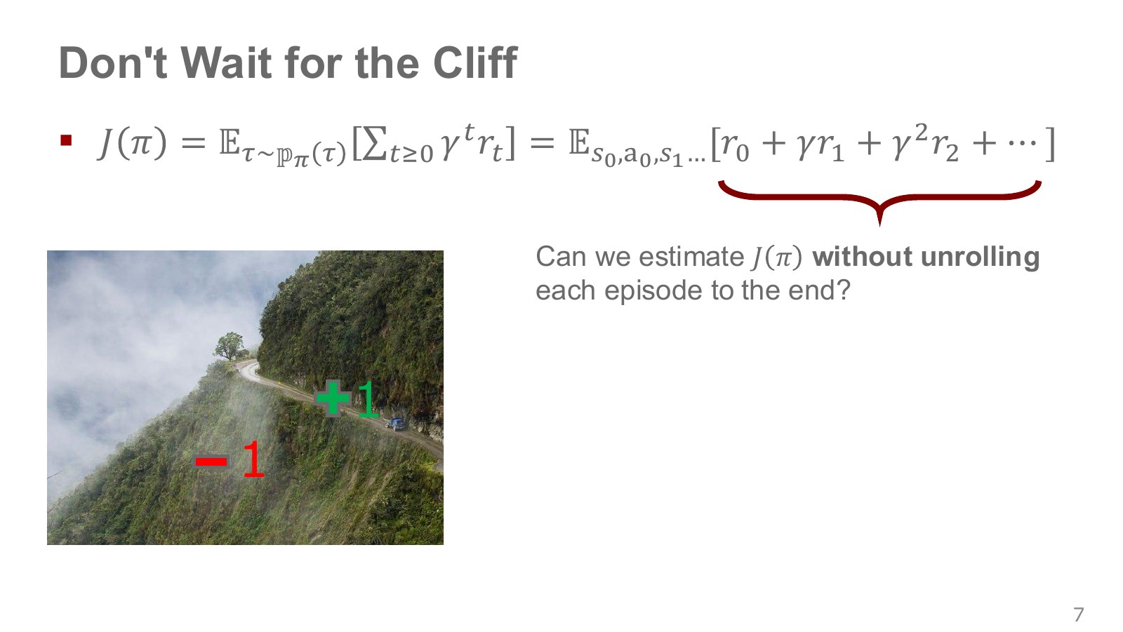
Measuring all of requires waiting for a complete rollout. That is intuitive, but updates are delayed in tasks whose consequences arrive much later.
Instead, combine reward received now with an estimate of rewards still to come from the next state. A value function supplies that estimate. The key is being able to update before the execution ends.
This does not reveal a cliff’s danger automatically without experience. Future-value estimates must come from a model or earlier data, and can be wrong. A computational method for learning before an episode ends is distinct from operational measures preventing hazardous exploration on real equipment.
#P009 · A value function averages future rewards from the current state
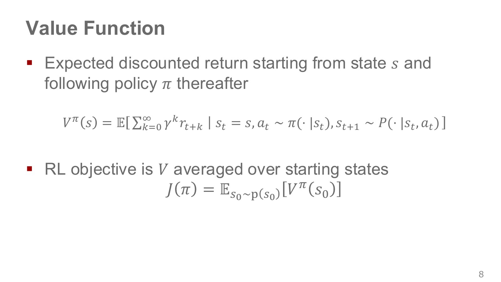
is the expected return starting in state and subsequently following policy . Superscript identifies the policy being evaluated; it is not an exponent.
Explore the symbols and calculation State value is the expected sum of future discounted rewards when following a particular policy from that state
Read the equation in words
This is a long-term score for continuing with a policy from a given state. Even a small immediate reward can lead to high value if good outcomes follow later.
Understand each symbol
- State value: the average return obtained by starting in a state and continuing to follow the policy.
- The state at step , containing information such as position and velocity needed to predict what happens next.
- The discount factor for future rewards. Zero considers only the immediate reward, while values near one give more weight to the distant future.
- The reward received at one step: a learning signal defined so that larger is better.
- Add every term over the indicated range, computing one term and repeating through the end of the range.
- An expectation: an average over possible outcomes weighted by their probabilities.
- Conditional notation: the information to the right of the bar is given. This is not a division sign.
Follow the calculation
- Starting with the current reward, apply each time step's discount weight and add the terms.
- Average over the possible futures from that state.
Check with a small example
With reward 0 now, reward 10 next, and discount factor 0.9, those two steps contribute 9. This can be better than an action that gives 1 immediately and ends.
An illustrative example for understanding the equation.
A state close to a cup can still have low value under a policy that moves the gripper incorrectly. Value is therefore not a location’s intrinsic score: environment, reward, discounting and policy determine it together. It is generally different from success probability and can be negative or greater than one.
With starts sampled from distribution , overall performance averages state values as . This connects an expectation from one state to average performance across an experiment.
#P010 · The Bellman expectation equation: connect current reward to next-state value
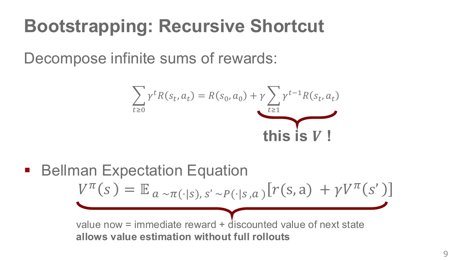
Separate the first reward from the future sum, and the remaining terms share one discount factor. This simple decomposition turns a long-horizon problem into a one-step recursive relationship.
Explore the symbols and calculation The Bellman expectation equation averages over both policy actions and the environment's next states
Read the equation in words
Current value equals the average of immediate reward plus discounted next-state value. The equation averages over uncertainty in both action selection and environment transitions.
Understand each symbol
- State value: the average return obtained by starting in a state and continuing to follow the policy.
- A policy choosing actions given a state. A stochastic policy outputs probabilities or probability densities for actions.
- The probability of a next state after acting in the current state, or its density for continuous states.
- The discount factor for future rewards. Zero considers only the immediate reward, while values near one give more weight to the distant future.
- The reward term actually used depends on the current state, action, and next state.
- Add every term over the indicated range, computing one term and repeating through the end of the range.
- Conditional notation: the information to the right of the bar is given. This is not a division sign.
Follow the calculation
- For each action, calculate reward and future value for the possible next states.
- Average using environment probabilities, then average again using the policy's action probabilities.
Check with a small example
If an action certainly gives reward 1 and reaches a state with value 4, a discount factor of 0.5 gives a one-step evaluation of .
An illustrative example for understanding the equation.
The outer sum averages actions chosen by the policy; the inner sum averages next states the environment can produce after each action. Counting the current reward again inside next-state value would double-count it. Here summarizes rewards after arriving in the next state.
Using a current estimate to construct another estimate is bootstrapping. With next value 0.8, immediate reward 0.2 and discount factor 0.9, the one-step target is 0.92. After genuine task termination, there are no further rewards and the future term is zero.
Silver’s dynamic-programming lecture, from 13:00 also turns Bellman relationships into iterative calculations. Distinguish the relationship among true values from the algorithm repeatedly updating provisional values to obtain them.
#P011 · Knowing optimal values lets us choose the next action
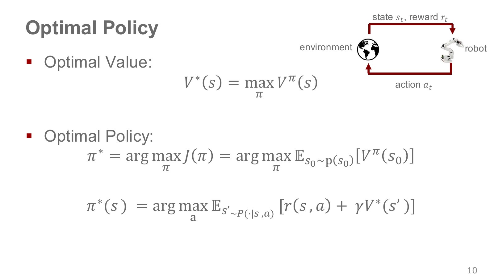
Unlike for a fixed policy, is the best value over policies. If we already know it, choose the action maximizing immediate reward plus discounted next optimal value.
Explore the symbols and calculation The Bellman optimality equation makes a one-step choice that includes optimal future performance
Read the equation in words
The equations define both the value obtained by choosing the best action in each state and the policy that chooses it. Distinguish the highest score from the action producing it.
Understand each symbol
- The probability of a next state after acting in the current state, or its density for continuous states.
- The discount factor for future rewards. Zero considers only the immediate reward, while values near one give more weight to the distant future.
- The state value and policy under optimal choices.
- Respectively, the largest value and an action attaining it.
- Add every term over the indicated range, computing one term and repeating through the end of the range.
- Conditional notation: the information to the right of the bar is given. This is not a division sign.
- Select the input attaining the largest or smallest value, rather than the value itself.
Follow the calculation
- For each action, average immediate reward plus the optimal value of the next state.
- Use the maximum as the optimal value and an action attaining it as the optimal policy.
Check with a small example
If two actions have long-term scores of 3 and 5, the optimal value is 5 and the policy chooses the second action.
An illustrative example for understanding the equation.
The first line gives the maximum value; the second gives an action attaining it. Membership symbol allows tied actions. Read these equations under the finite-state, finite-action discounted-MDP assumptions used here.
This is not a shortsighted rule choosing only the largest immediate reward: the next-state value contains the longer future. A push with no reward now can still have high value if it makes a later grasp easier.
#P012 · Value iteration: from an empty table toward optimal values
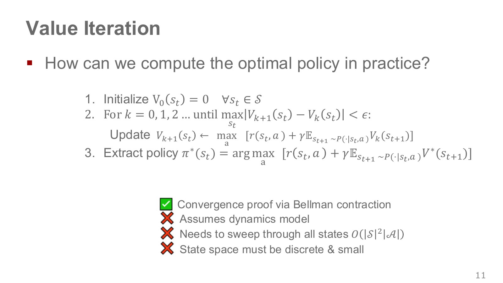
Value iteration initializes state values simply—for example, all zeros—and repeatedly evaluates the right-hand side of the Bellman optimality relationship.
Explore the symbols and calculation Value iteration uses the previous iteration's values to compute the best one-step target for each state
Read the equation in words
Compute a new value table from the current table. Repeatedly propagating future-value estimates brings value iteration closer to the optimal value.
Understand each symbol
- The probability of a next state after acting in the current state, or its density for continuous states.
- The discount factor for future rewards. Zero considers only the immediate reward, while values near one give more weight to the distant future.
- An index counting terms or repetitions. Check whether it denotes time steps or learning iterations in the equation.
- The value tables at the previous and next computational iterations. Here, is not actual environment time.
- Add every term over the indicated range, computing one term and repeating through the end of the range.
- Conditional notation: the information to the right of the bar is given. This is not a division sign.
Follow the calculation
- Hold the previous table fixed and compute a one-step score for every action.
- Write the largest score as each state's new value, then continue to the next iteration.
Check with a small example
If all future values start at zero, the first update includes only immediate rewards. Later iterations propagate the influence of rewards one step farther away.
An illustrative example for understanding the equation.
One sweep updates every table state once. A synchronous sweep reads the old table throughout and writes a new table. Increasing does not mean the real robot took a step; it counts computations using the model.
For a finite discounted MDP, this operation has a contraction property: the largest difference between two value tables shrinks by at most factor . Repetition approaches the same fixed point, the optimal value. The same guarantee does not automatically cover every problem with discount factor one.
When the largest table change is small enough, stop and extract the best actions. Summing all next states through a dense transition matrix costs roughly per sweep. Sparse transitions with few feasible next states can be cheaper. With a small state set and known model, this makes a useful reference solution.
#P013 · Reading numbers, colors and arrows separately in a grid
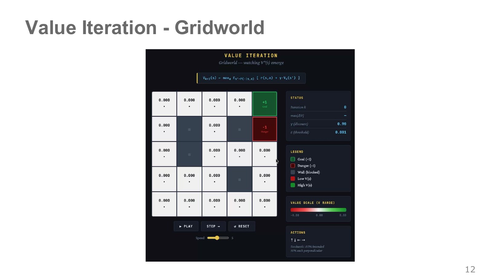
Green marks the goal, red danger and gray walls. Numbers in the white cells estimate future discounted rewards from those states; arrows show actions chosen from those estimates. Color visualizes value magnitude, not visitation count or success probability itself.
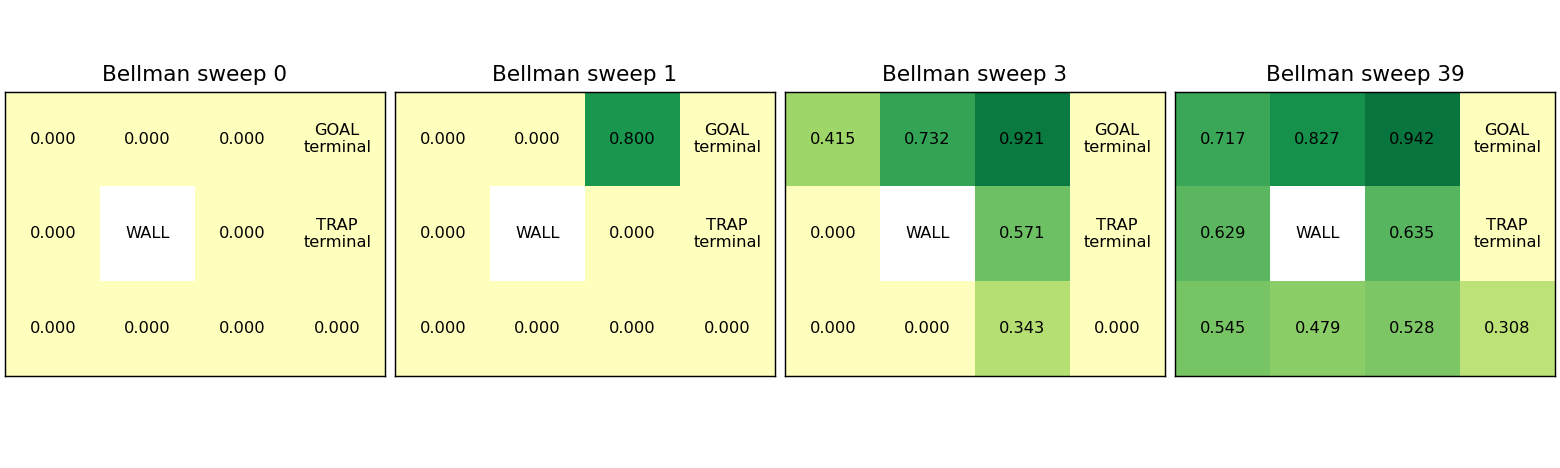
The source demo moves in the intended direction with probability 80% and to either side with 10% each. Handling walls and boundaries is also part of the transition model. Starting from zeros, values appear near the goal first because one sweep passes future-reward information one transition backward.
The following is a separate 3×4 environment I made to check the same principle. Entering the goal gives +1 and entering danger −1, then terminates the episode. Thus future value after entering a terminal cell is zero. This convention keeps the goal’s +1 entry reward distinct from its subsequent value.
#P014 · Policy evaluation: calculate the performance of the policy we have
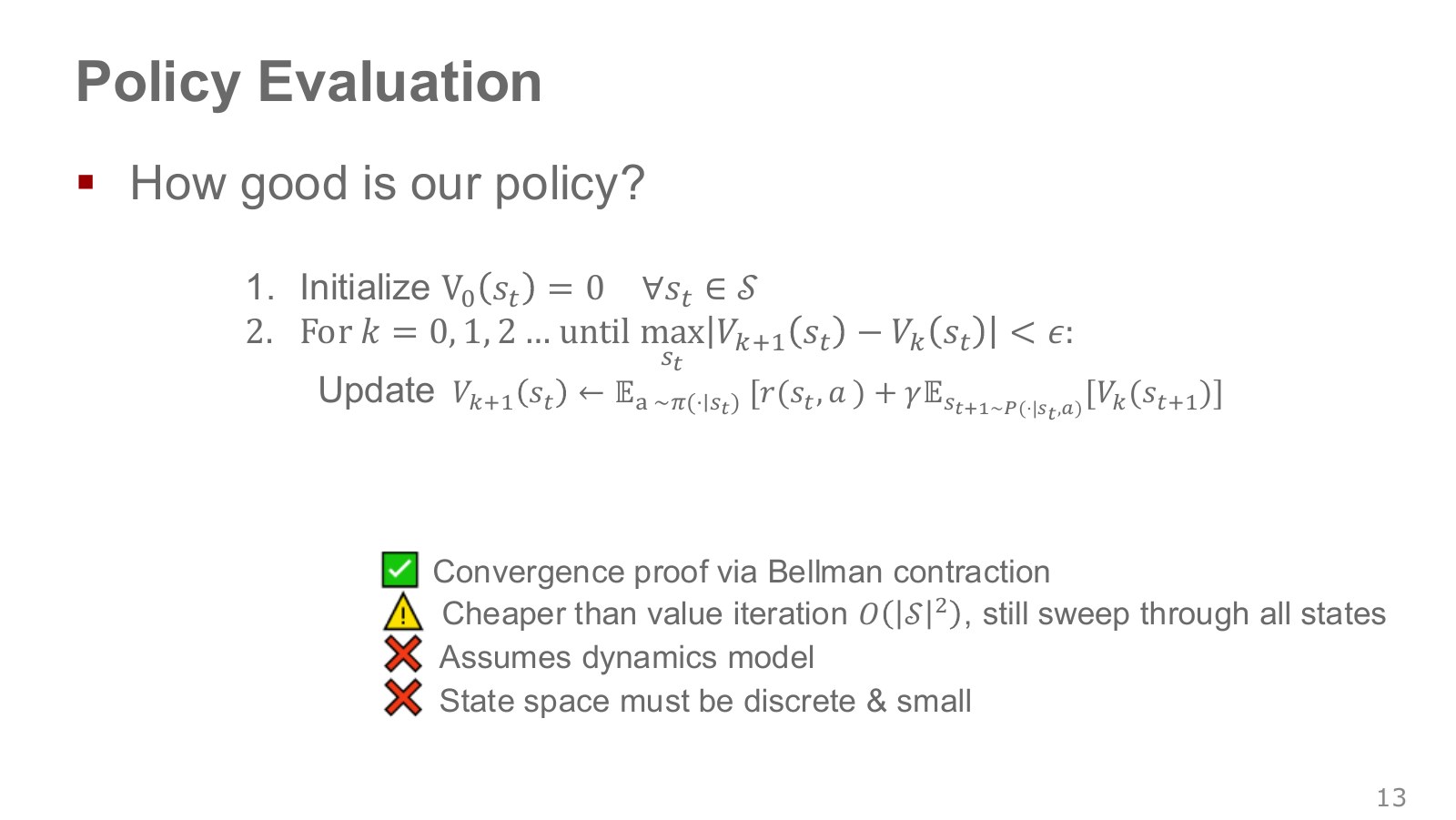
Now keep actions unchanged and ask how well a specified policy performs. Policy evaluation averages the actions that policy actually takes instead of selecting the best one.
Explore the symbols and calculation Policy evaluation repeatedly updates values using weighted averages under a fixed policy's action probabilities
Read the equation in words
Keep the policy unchanged and calculate only its score. Instead of taking a maximum as in value iteration, average according to how often the policy actually chooses each action.
Understand each symbol
- A policy choosing actions given a state. A stochastic policy outputs probabilities or probability densities for actions.
- The probability of a next state after acting in the current state, or its density for continuous states.
- The discount factor for future rewards. Zero considers only the immediate reward, while values near one give more weight to the distant future.
- An index counting terms or repetitions. Check whether it denotes time steps or learning iterations in the equation.
- The policy-value estimate from the previous iteration.
- Add every term over the indicated range, computing one term and repeating through the end of the range.
- Conditional notation: the information to the right of the bar is given. This is not a division sign.
Follow the calculation
- Hold the current policy's action probabilities fixed.
- Repeatedly update only the value table, averaging reward plus discounted next value under those probabilities.
Check with a small example
If left and right have scores 2 and 6 and the policy chooses each half the time, the new value is 4. This differs from maximizing by choosing only the better score, 6.
An illustrative example for understanding the equation.
Suppose two actions have one-step expected outcomes 0 and 1, and the policy selects each half the time. Evaluation gives 0.5. Maximizing instead would give 1, but answers a different question from evaluating the current policy.
The figure’s “cheaper” description also depends on implementation. For a deterministic policy, or with policy-averaged transitions and rewards precomputed, a sweep can be counted as . Explicitly summing every action of a stochastic policy retains action-count costs. Replacing a maximum with an average does not remove all action computations in every implementation.
#P015 · A maximum and a policy average answer different questions
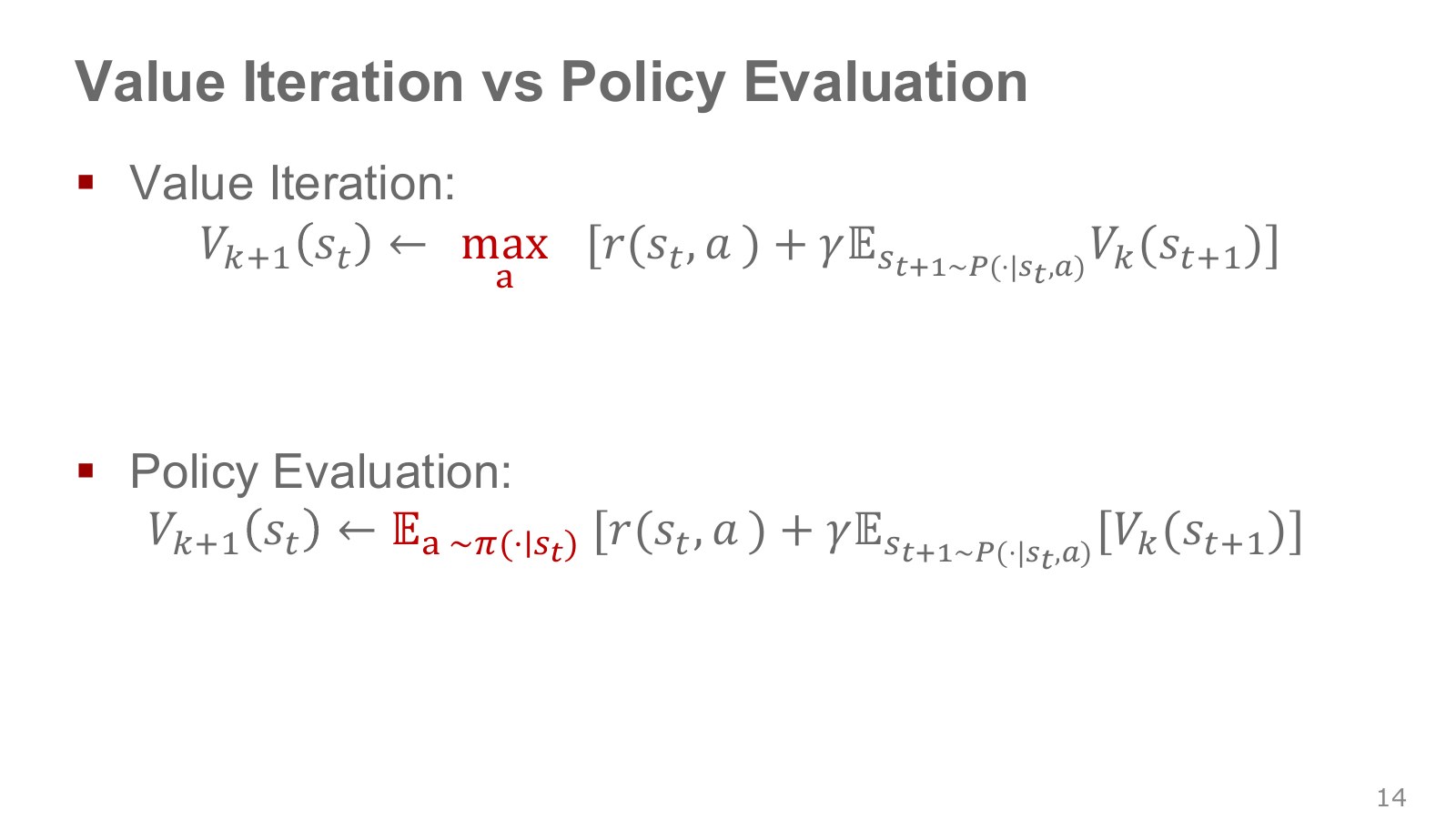
The red asks what happens if we choose the best action from now on. The red asks what happens if we behave according to an already specified policy. Both use next-state values, but differ in the rule determining the current action.
For example, suppose moving directly toward a cup has expected outcome 0.8 and detouring has 0.6. A policy choosing both equally gives evaluation 0.7, whereas maximization gives 0.8. These numbers are a separate illustration of the distinction.
This is why policy evaluation and value iteration should not be memorized as the same algorithm merely because their equations look similar. First identify what stays fixed and what improves; policy iteration then follows naturally.
#P016 · Policy iteration: evaluate, then improve using that evaluation
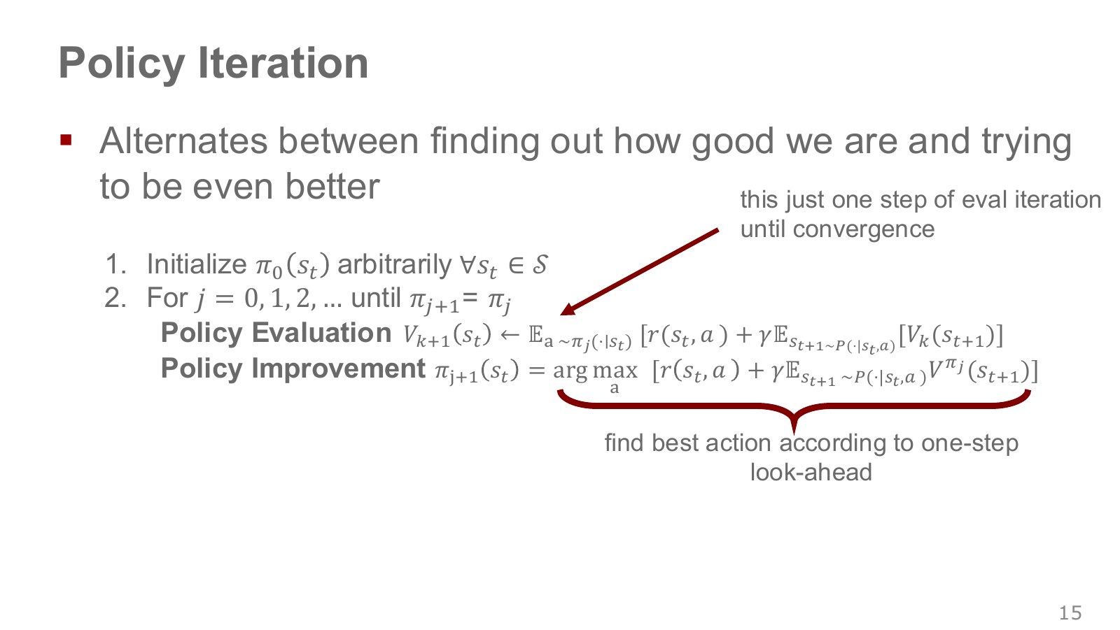
Policy iteration alternates two operations. First evaluate the current policy sufficiently to obtain , then choose better one-step actions using those values.
Explore the symbols and calculation Policy improvement selects better actions using the future values of the current policy
Read the equation in words
Improve the first action using future values computed for continuing with the current policy. Alternate policy evaluation and policy improvement.
Understand each symbol
- The probability of a next state after acting in the current state, or its density for continuous states.
- The discount factor for future rewards. Zero considers only the immediate reward, while values near one give more weight to the distant future.
- The policies before and after improvement. Here, indexes policy-improvement iterations.
- Future value when following the current policy.
- Add every term over the indicated range, computing one term and repeating through the end of the range.
- Conditional notation: the information to the right of the bar is given. This is not a division sign.
- Select the input attaining the largest or smallest value, rather than the value itself.
Follow the calculation
- First evaluate the current policy's value.
- Use those future values to score each action, then change the policy to choose the highest-scoring action.
Check with a small example
If the current policy chooses an action scoring 2 while another action has a one-step improvement score of 3, replace the action in that state with the second one.
An illustrative example for understanding the equation.
counts policy changes, distinct from counting the inner value-evaluation iterations. One evaluation line in the source abbreviates a calculation usually repeated to convergence. Variants improving after just one evaluation step relate to generalized policy iteration, but differ from the exact evaluation described here.
In a finite discounted MDP, exact evaluation followed by greedy improvement makes value no worse. It need not strictly increase every state’s value or the return from a particular start at every iteration: actions may tie or already be optimal. A consistent tie rule, such as retaining the current action, reduces needless policy changes.
Silver’s evaluation–improvement explanation, from 35:40 separates the same two questions. Instead of differentiating a loss once, we sum model probabilities to calculate values and then change the policy.
#P017 · Alternating policy-evaluation and policy-improvement screens
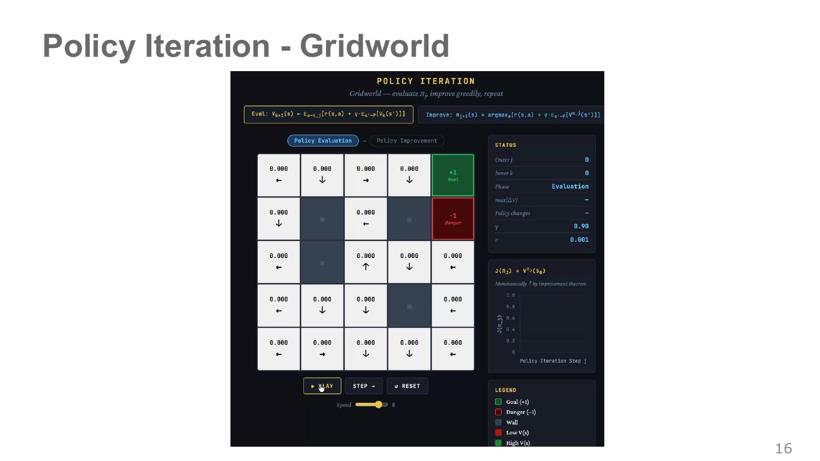
The two steps above are evaluation, which calculates numbers while keeping arrows fixed, and improvement, which changes arrows using those numbers. Changing values during evaluation does not mean a new policy has been executed.
The return graph on the right summarizes something different from the value tables over sweeps. Its interpretation requires knowing the starting distribution over which performance was averaged. A graph immediately after initializing provisional values to zero should not be equated with actual performance of a converged policy.
In my example, I solved policy evaluation exactly as a small linear system and compared all nonterminal state values before and after improvement. I separately checked nondecreasing values and agreement with the final value-iteration solution. This makes the comparison more explicit than simply observing that a graph rises.
#P018 · Acting from state values requires more calculation of consequences
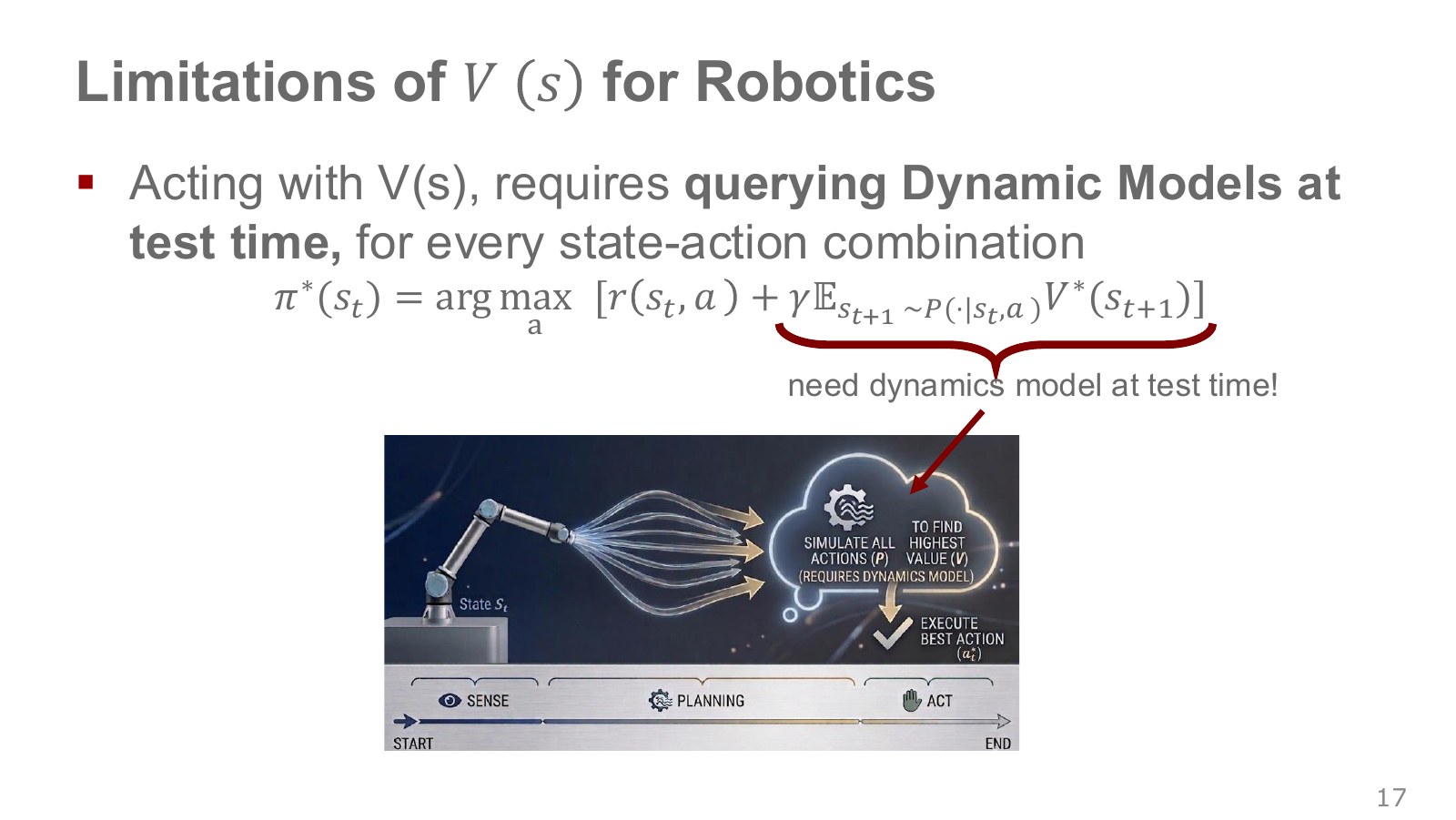
scores states. Choosing a current action requires comparing possible next states and their values for each action. The hypothetical arm trajectories feeding into the planning box illustrate that additional computation.
This one-step lookahead needs queries to reward and transition model . Models can be inaccurate under complex contact and friction, and slow calculations can miss the next control deadline. Learning state values does not make action selection free.
This is not an absolute rule that a value-iteration policy must run the model again at deployment. A small tabular problem can store the best actions in advance. The limitation here concerns computing actions from state values on demand.
#P019 · A Q function specifies the first action as well as the state
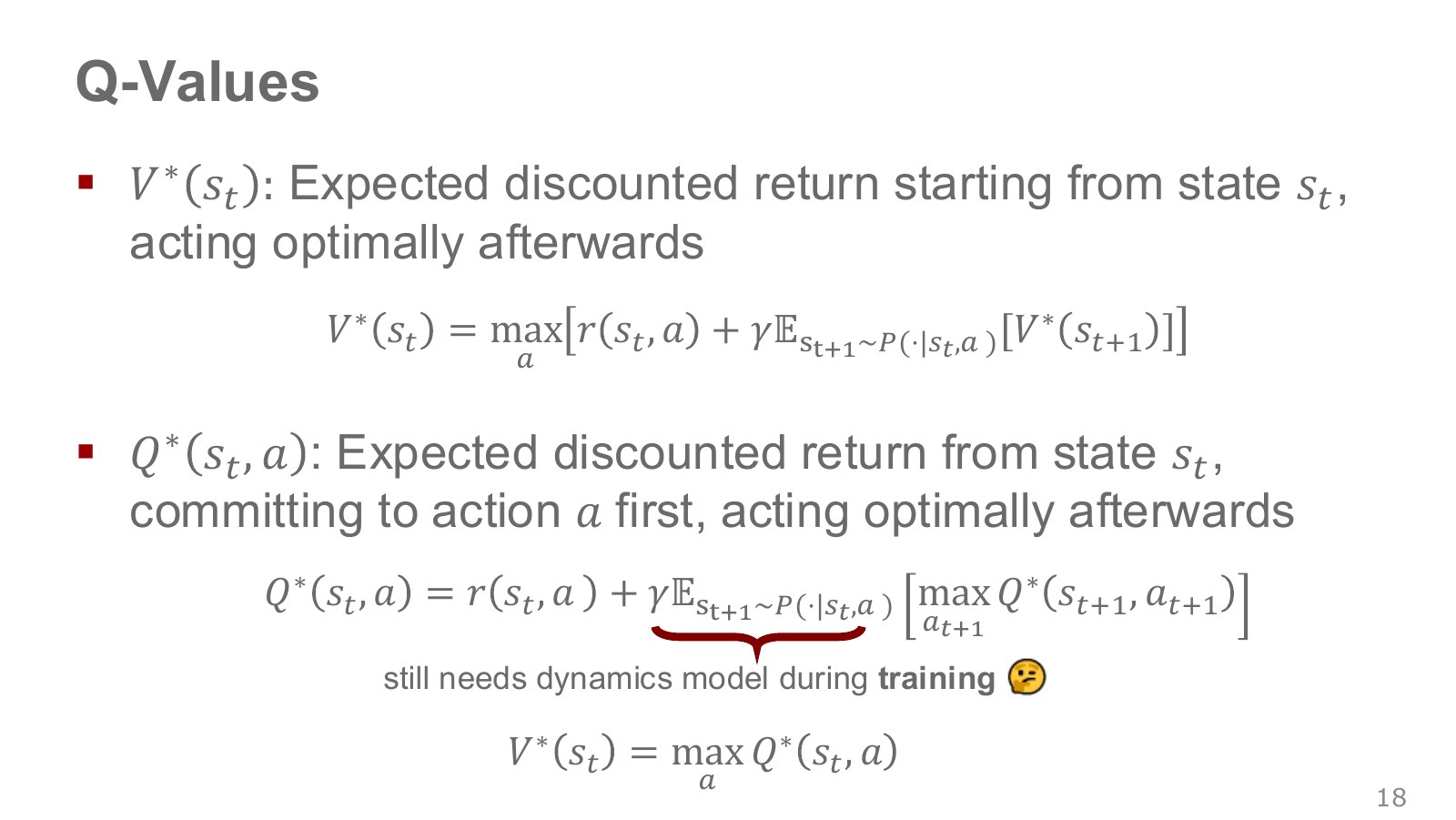
is expected return from the current state when only the first action is fixed to and policy is followed afterward. It takes one additional action input compared with . Starred assumes optimal behavior after that first action.
Explore the symbols and calculation Optimal action value combines the first action's outcome with optimal action values in the next state
Read the equation in words
Define long-term value with a particular first action specified. From the next state onward, assume the best actions are selected.
Understand each symbol
- The probability of a next state after acting in the current state, or its density for continuous states.
- The discount factor for future rewards. Zero considers only the immediate reward, while values near one give more weight to the distant future.
- Optimal action value with the first action specified.
- Optimal state value before choosing an action: the maximum over all action values.
- Add every term over the indicated range, computing one term and repeating through the end of the range.
- Conditional notation: the information to the right of the bar is given. This is not a division sign.
Follow the calculation
- Calculate the first action's reward and next state.
- Add the discounted maximum next-state action value, then average over environment probabilities.
Check with a small example
With first reward 1, best next-state action value 8, and discount factor 0.5, the first action's value is 5.
An illustrative example for understanding the equation.
is an action considered in the next state, distinct from the currently executed . “Move 1 cm left in front of the cup” and “move 1 cm right” can have different values. A good function compresses which commands are favorable over the long term.
-value iteration directly repeats this equation using a transition model during computation. A function itself does not inherently require a model; Q-learning below learns the same relationship from sampled experience.
#P020 · With Q values available, execution compares actions at the current state
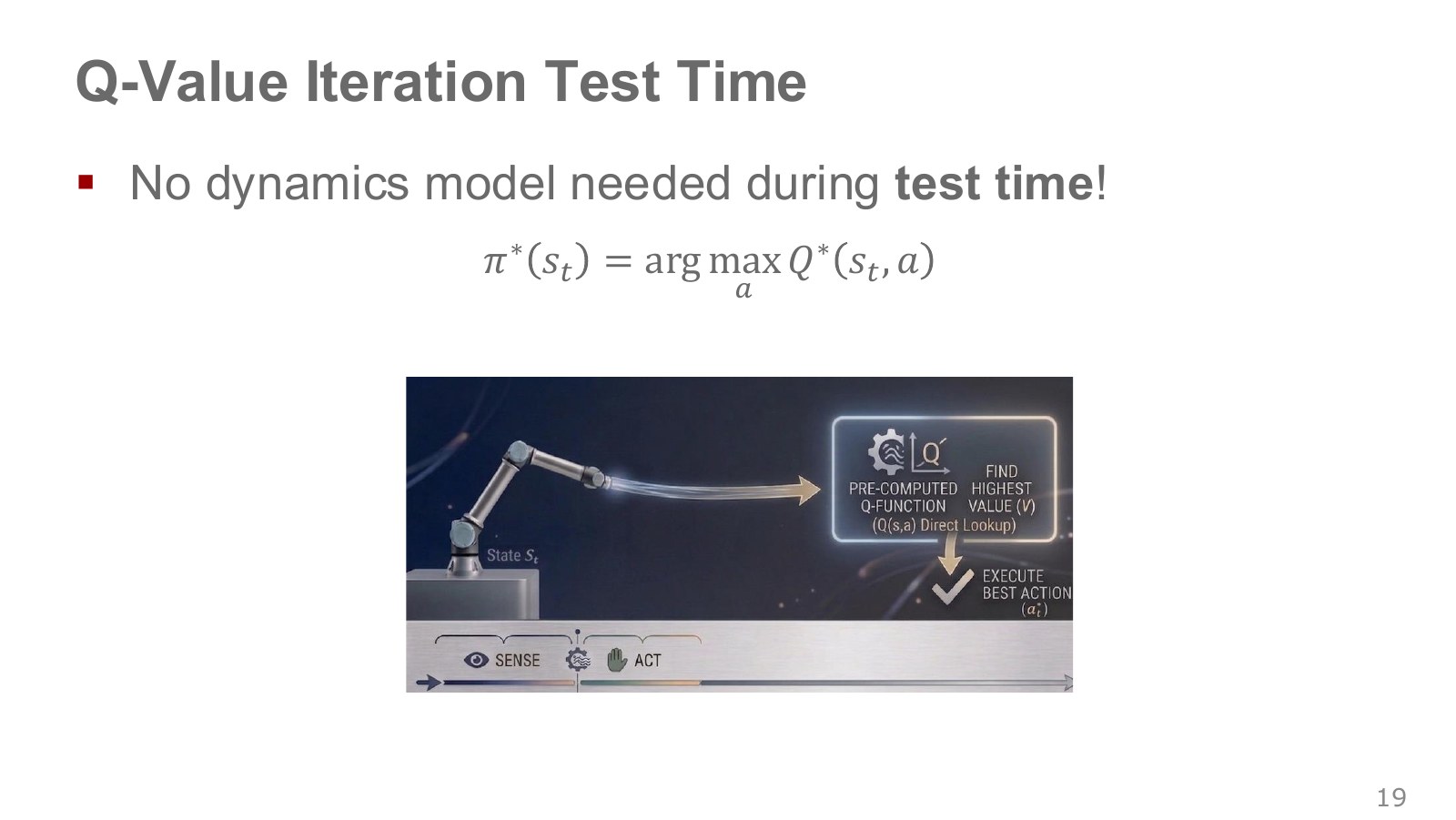
For finitely many actions, read their values and select an action attaining the largest.
Explore the symbols and calculation A greedy policy selects the action with the largest currently estimated action value
Read the equation in words
The greedy policy chooses the action that looks best under the current estimates. Inaccurate values can lead to an incorrect choice.
Understand each symbol
- Action value: the average return obtained by taking a particular action in the current state and then following the policy.
- Select the input attaining the largest or smallest value, rather than the value itself.
Follow the calculation
- Compare the estimated values of the actions available in the current state.
- Choose an action attaining the largest value. Ties can be handled with a separately specified rule.
Check with a small example
For estimated action values [1, 4, 2], choose the second action. Repeating only this rule can miss good actions that have not yet been tried.
An illustrative example for understanding the equation.
The shorter flow below evaluates an already learned function instead of simulating transitions at deployment. Greedy means maximizing the estimate. Because contains longer-term consequences, it does not mean seeking only immediate reward.
An incorrect estimate can still produce an incorrect choice. With continuous actions, listing every candidate is impossible, so itself becomes difficult. A one-line equation does not remove computational cost; CEM and DDPG later address this problem.
#P021 · Q-learning: update from observed transitions instead of model averages
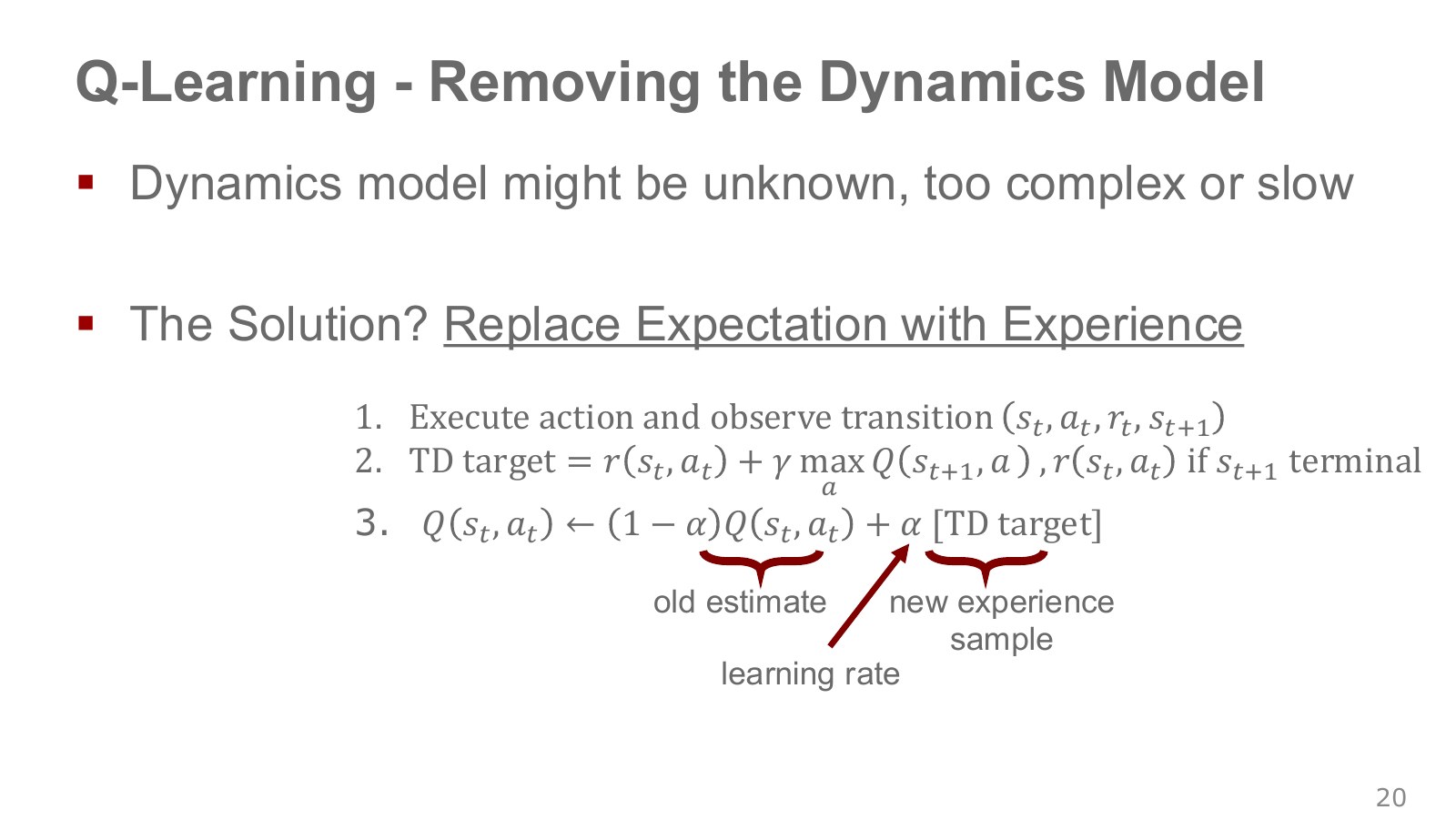
Q-learning uses environmental samples . Instead of summing every possible next state, it constructs an update target from the one actually observed. TD, or temporal difference, connects a current estimate with the next step’s reward and estimate.
Explore the symbols and calculation Q-learning updates one table entry using the difference between its current value and a TD target that accounts for termination
Read the equation in words
Use one observed transition to adjust one action-value table entry. Move from the current estimate toward the target by the learning-rate fraction.
Understand each symbol
- The state at step , containing information such as position and velocity needed to predict what happens next.
- The action chosen at step : for example, a torque, a joint target or a movement direction, depending on the setup.
- The reward received at one step: a learning signal defined so that larger is better.
- The discount factor for future rewards. Zero considers only the immediate reward, while values near one give more weight to the distant future.
- An indicator equal to 1 for actual termination and 0 otherwise. It prevents adding future value after termination.
- The training target that the current prediction should approach. It may be a fixed label or a value constructed from another estimate.
- The TD error: the difference between the one-step target and the current value estimate.
- The learning rate setting the update size. A large value can move faster but destabilize the iteration.
Follow the calculation
- If the transition is nonterminal, add the discounted maximum next-state value to the reward.
- Subtract the current estimate from the target to obtain the TD error, then add a fraction of it to the current estimate.
Check with a small example
With current value 2, reward 1, next maximum 4, and discount factor 0.5, the target is 3. A learning rate of 0.1 gives a new value of 2.1. On termination, the target is just 1.
An illustrative example for understanding the equation.
marks genuine task termination, removing the future term. is the TD error and the learning rate setting update size. Other state–action entries stay unchanged in this individual tabular update.
With current value 0.4, reward 0.2, next maximum 0.8, discount factor 0.9 and learning rate 0.25, the target is 0.92 and updated value 0.53. At task termination, the target is just 0.2 and the new value 0.35. Distinguish reward from target, and target from the updated estimate.
One transition samples a Bellman target based on current ; it is not an exact label already equal to true optimal value . Next-state estimation errors enter the target too. An externally truncated rollout can differ from genuine task termination, so implementations must distinguish them when defining the future term.
#P022 · Calculating every cell with a model versus learning the cells experienced
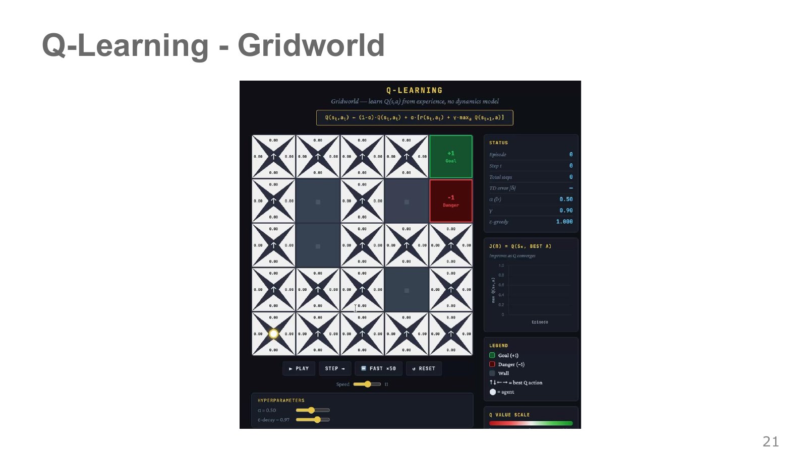
Each cell’s four triangles represent estimates for the four directional values. Value iteration displayed one best value per state; Q-learning maintains separate action values within the same cell. Values near explored routes therefore change first.
Repeatedly choosing only what currently looks best may miss other actions’ benefits. Exploration tries less certain actions to gain information; exploitation selects actions already estimated to be good. -greedy provides a simple compromise by choosing randomly with a specified probability.
Neither using learning rate 0.1 nor running for a long time alone guarantees convergence. Typical tabular finite-discounted guarantees require state–action coverage, sufficient visits and suitable decreasing learning rates. Data never reaching an unfamiliar state cannot establish its best actions.
#P023 · Off-policy learning: separate the collection policy from the policy being learned
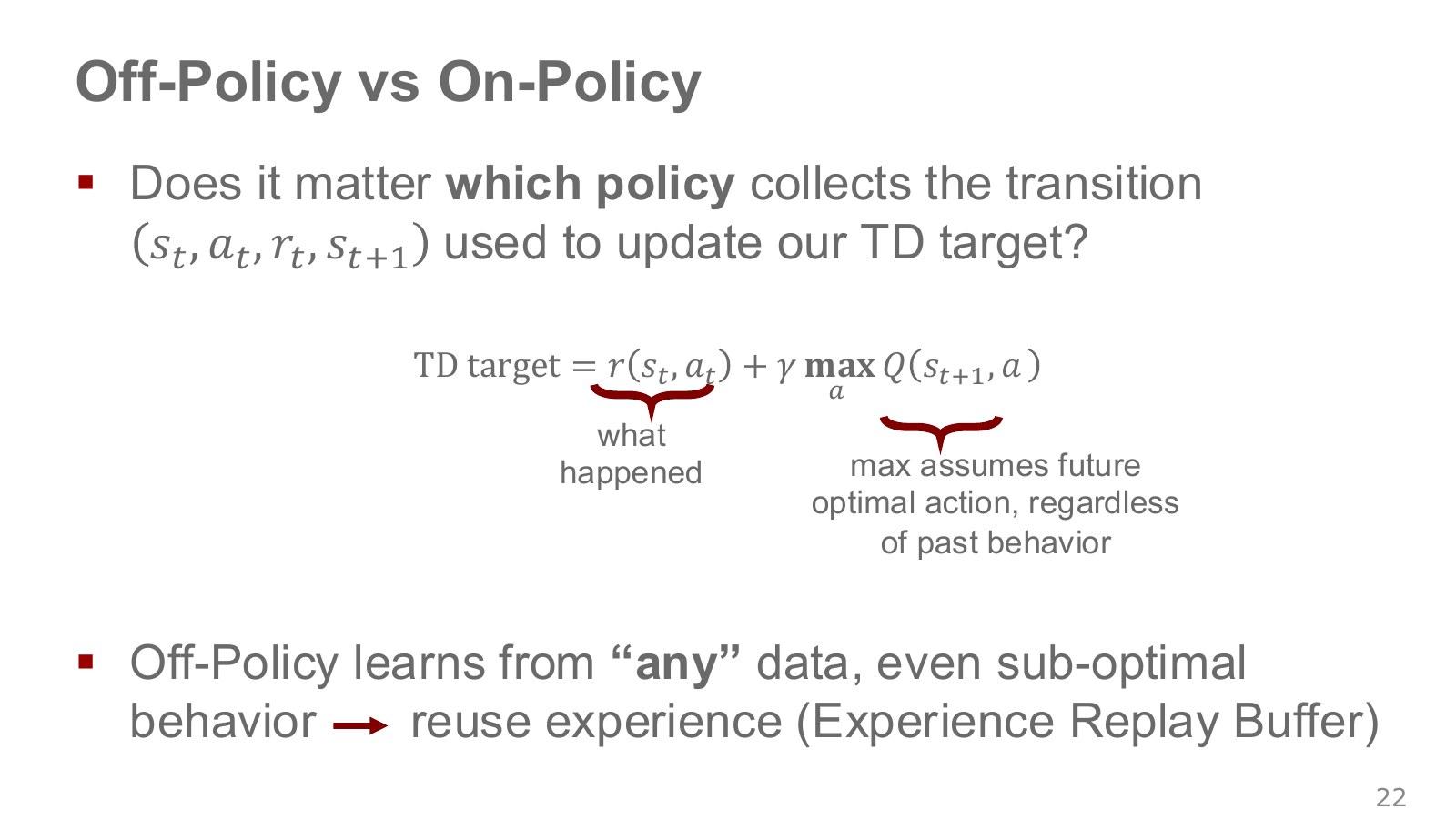
The behavior policy chooses actions while collecting real transitions. The target policy is the rule currently being evaluated or improved. Learning that permits them to differ is off-policy.
Q-learning uses the action actually taken and reward received, but assumes the next step takes the best action under current . This permits reusing records from older or exploratory policies. This target-policy distinction differs from the target network discussed later.
Being able to reuse data does not mean quality and coverage can be ignored. Transitions must be valid for the same environment and reward definition; unobserved actions leave their values uncertain. Networks assigning exaggerated values to unseen actions become particularly important in offline reinforcement learning.
Silver on on-policy and off-policy learning, from 4:10 also distinguishes whether the followed behavior matches the behavior being learned. Using someone else’s records does not make the objective imitation learning: the update here uses recorded rewards and future values.
#P024 · SARSA: use the value of the next action actually selected
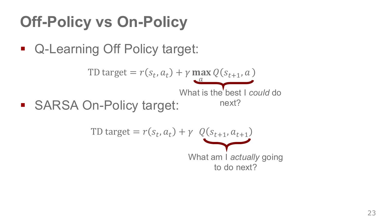
SARSA takes its name from State–Action–Reward–State–Action. It uses the next action chosen by the current behavior policy after arriving in the next state.
Explore the symbols and calculation Q-learning uses the maximum next-action value; SARSA uses the value of the next action actually selected by the current policy
Read the equation in words
Even for the same transition, targets differ according to what action is assumed to follow. Q-learning uses the best next action, while SARSA uses the action selected by the actual policy.
Understand each symbol
- The reward received at one step: a learning signal defined so that larger is better.
- The discount factor for future rewards. Zero considers only the immediate reward, while values near one give more weight to the distant future.
- An indicator equal to 1 for actual termination and 0 otherwise. It prevents adding future value after termination.
- Action value: the average return obtained by taking a particular action in the current state and then following the policy.
- The next action actually selected by the current behavior policy.
Follow the calculation
- Use the same reward, discount factor, and termination indicator in both equations.
- Q-learning reads the next maximum; SARSA reads the value of the actual next action.
Check with a small example
If next-action values are 5 and 1 but exploration selects the second action, the future terms use 5 and 1 respectively. This is why the algorithms differ.
An illustrative example for understanding the equation.
Suppose next-state action values are 0.8 and −0.4, but exploration selects the second action. Q-learning uses 0.8 in its target, while SARSA uses −0.4. SARSA learns the consequences of the current policy including its exploratory behavior.
The source contrasts “what is best possible” with “what will actually happen next.” Q-learning also issues real commands to collect experience. The distinction is which policy’s action enters the future-value calculation, not whether the robot physically acts.
#P025 · Cliff-edge and detour routes: the cost of exploratory mistakes
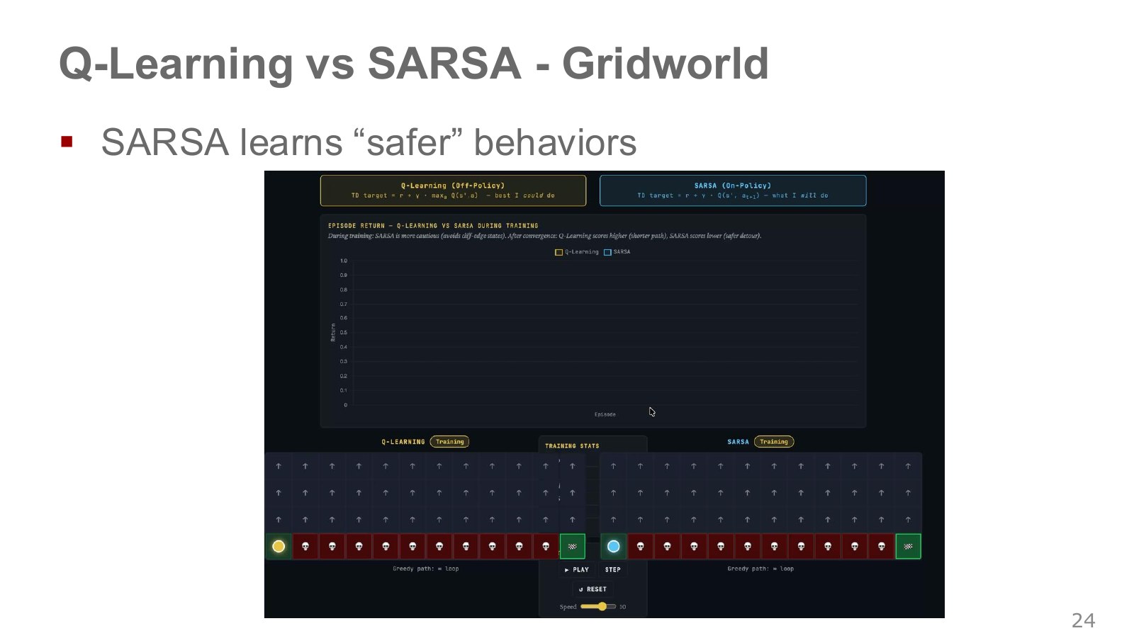
Both grids start at the bottom left and aim for the bottom-right goal. The red strip is a cliff. The route above it is short, but one mistaken downward move incurs a large loss. A detour takes more steps but is less sensitive to exploration errors.
Imagine a training policy that occasionally moves into an adjacent cell. The cliff-side route can be shortest once exploration is disabled. While exploration continues, falling costs more than stepping away from the edge, so SARSA may assign higher value to a detour.
SARSA evaluates persistent exploration errors as part of the current policy and can therefore favor a route farther from the edge in this setting. Q-learning’s target assumes the next action is best, so its values can favor the shorter route under greedy evaluation.
This does not guarantee that SARSA is always safe or Q-learning always risky. Outcomes depend on whether exploration decays, transitions themselves slip, and falls terminate the task or return to the start. Distinguish actual training-time behavior performance from evaluation with a fixed greedy policy.
#P026 · Two axes for the methods so far
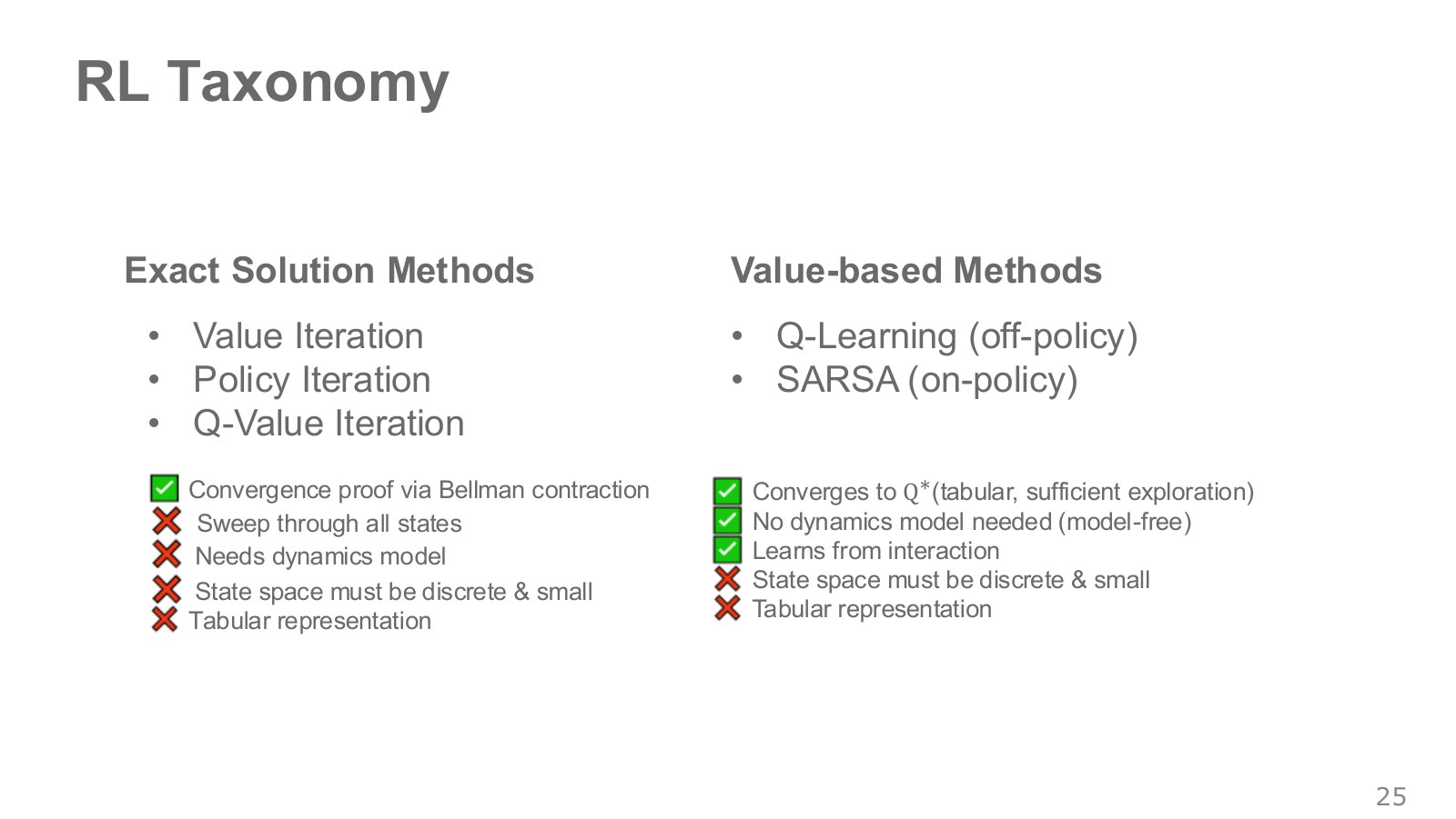
On the left is dynamic programming, which uses a known model to calculate possible next states. It breaks a large problem into overlapping smaller ones and reuses their solutions. Here we learned it through tables storing state values.
On the right are model-free methods updating values from transition samples, without explicitly learning or querying a next-state predictor. This does not mean physics is absent or simulation forbidden: simulated experience can train a model-free method.
Value iteration also uses values, so the diagram’s columns collect the algorithms discussed rather than defining completely exclusive philosophies. Do not replace tabular Q-learning’s convergence conditions and SARSA’s policy-change conditions with a blanket rule that enough exploration always guarantees optimality.
#P027 · Why we cannot create a table entry for every image
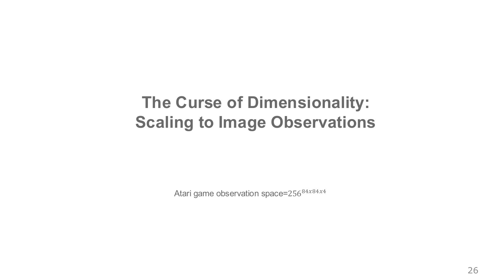
A grayscale pixel can take 256 values from 0 through 255. Stacking four 84×84 images gives the following enormous upper bound on pixel combinations.
Explore the symbols and calculation Enumerating pixel-value combinations as table entries makes the number of states grow exponentially
Read the equation in words
Storing every possible screen in a state table requires too many entries. The calculation multiplies the choices for each pixel across every pixel and frame.
Understand each symbol
- The 256 possible eight-bit pixel values, from 0 to 255.
- The number of input elements: frame height times width times the number of stacked frames.
Follow the calculation
- Count the elements in an input containing four stacked 84×84-pixel frames.
- Multiply the possibilities, assuming each element can take 256 values.
Check with a small example
Even two pixels yield possibilities. This is an upper bound on possible input combinations, not a claim that every screen actually occurs in the real world.
An illustrative example for understanding the equation.
Not every combination is a valid game scene. Even so, maintaining and sufficiently visiting independent entries for observed images is unrealistic. We need generalization: using what we learn in one scene in another.
Stacking four frames has another purpose: one image showing a ball’s position may not reveal whether it moves left or right. Several frames capture short-term change. A fixed frame count does not fully reconstruct hidden state in every environment.
#P028 · DQN: a network predicting action values from pixels
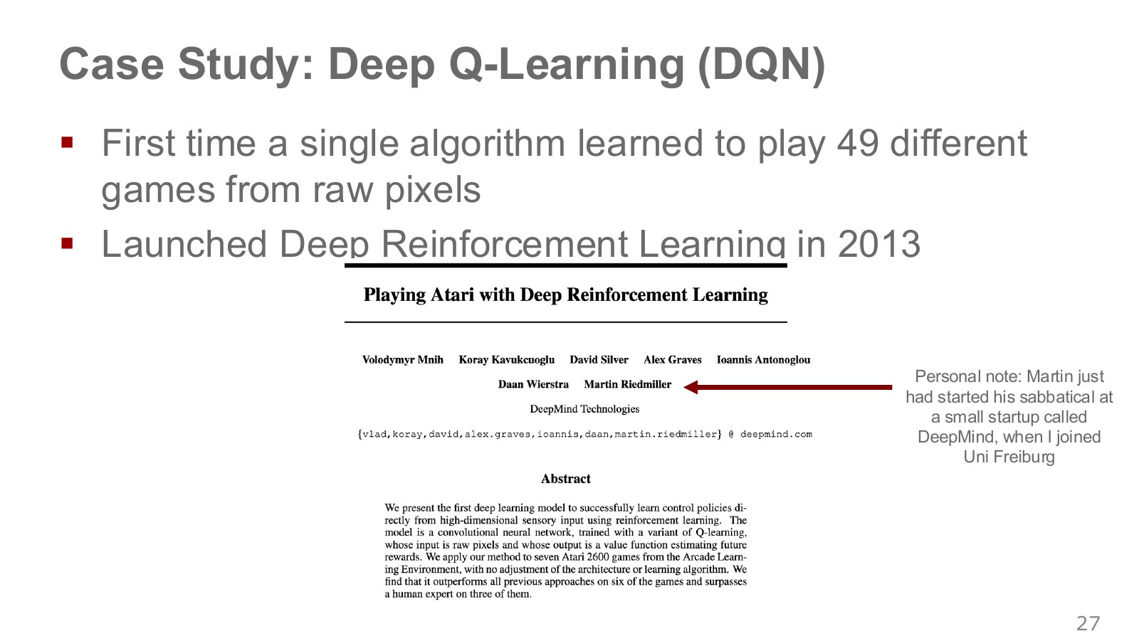
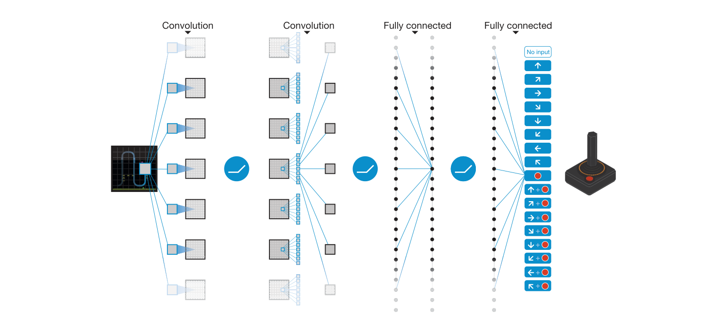
A Deep Q-Network (DQN) replaces a table with a neural network. Convolutional (CNN) layers read local image patterns, followed by feature-combining layers that output for each discrete action, such as left, right or fire. These are neither action-success probabilities nor classification probabilities.
The key was applying the same architecture and learning rules to multiple games. It did not mean one fixed set of weights mastered 49 games simultaneously: each game was trained separately. The source combines an image from the 2013 paper with a 49-game description, but the 2013 paper reports seven games and the 2015 Nature paper reports 49. Keep those scopes distinct.
Below is the architecture from the 2015 paper. Convolutional layers transform image patterns into features, while outputs on the right value each action-button combination. This differs from memorizing whole images independently in an exhaustive action table.
Original 2013 paper · Original 2015 paper.
#P029 · Reading DQN pseudocode through the movement of data
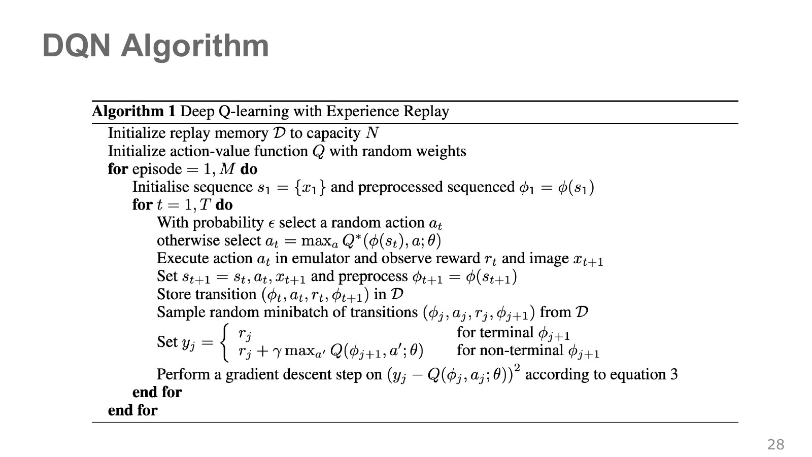
The small-print algorithm follows collect → store → sample → construct targets → update the network. denotes input preprocessing such as resizing, grayscaling and stacking frames. On this page, denotes the network weights.
- Initialize experience memory and the network.
- Choose an exploratory or best action from current . The action-returning operation is ; the maximum number itself is not a motor command.
- Obtain a game transition and store it in memory.
- Sample a minibatch from past transitions in memory.
- Construct a TD target for each sample and update weights to reduce squared differences between current predictions and targets.
A newly collected transition need not appear immediately in the next minibatch. Updating a tabular Q entry affects just that entry; updating shared network weights can also change outputs for other similar inputs. This sharing supports generalization but can also cause instability.
This page shows the 2013 pseudocode. Subsequent pages add stabilization with a separate target network. Following the data flow makes the memories and symbols understandable even where the lecture passed quickly over the algorithm.
#P030 · Experience replay: reuse a transition after collecting it
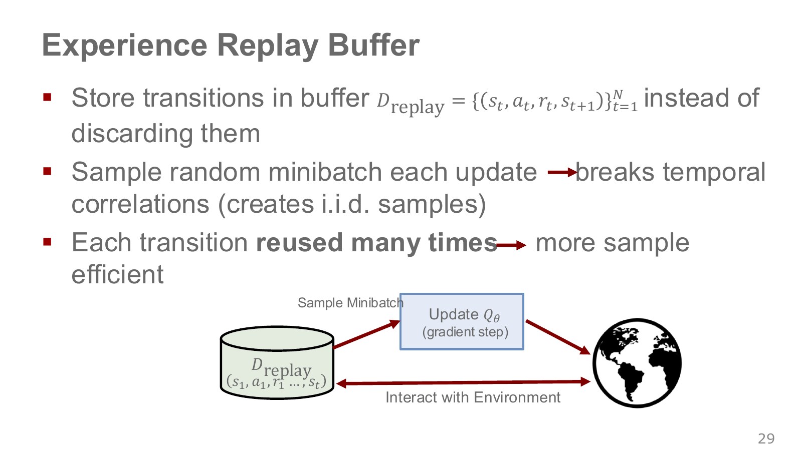
Cylinder is a replay buffer storing past transitions. Save experiences as they arrive, then sample records from different times for updates. One expensive real-world interaction can support several training updates.
Consecutive game frames repeat similar screens and actions. Mixing transitions from different times in a replay batch reduces concentration on one scene. Rare transitions can also be learned again while they remain in the buffer.
Training only on successive frames creates strongly similar inputs concentrated along a narrow visited route. Random sampling reduces temporal correlation and mixes update inputs. It does not make the stored distribution and visitation record perfectly independent and identically distributed: duplicates, changing buffer contents and changing policies remain.
Data reuse and adequate coverage are separate benefits. A buffer that never experienced the goal reward cannot invent success information by resampling. Off-policy learning reconnects here with exploration coverage.
#P031 · Target networks: when the number being fitted keeps moving too
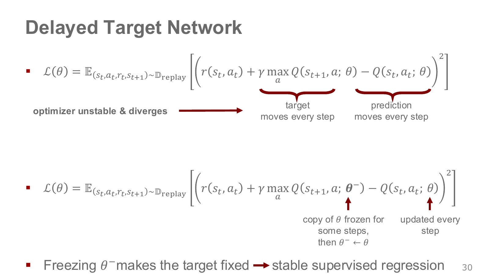
The upper expression uses one set of weights for both the current prediction and next-state target. Adjusting weights to correct the current value also changes next-state outputs, moving the target just fitted.
below denotes the target network weights. Copy the current learning network and hold that copy fixed for a period, separating the target-producing path.
Explore the symbols and calculation DQN constructs TD targets with a fixed target network and fits current predictions without differentiating through those targets
Read the equation in words
Use a separate target network to construct TD targets and fit the current network's predictions to them. Do not differentiate through the computation that creates the targets.
Understand each symbol
- Action value estimated by a neural network with these weights. It is not guaranteed to equal the true value.
- The separate network's value estimate used to compute targets. The superscript minus denotes delayed weights, not a negative number.
- The discount factor for future rewards. Zero considers only the immediate reward, while values near one give more weight to the distant future.
- An indicator equal to 1 for actual termination and 0 otherwise. It prevents adding future value after termination.
- The parameters collecting the trainable weights of the network or policy.
- The number of samples in one training minibatch.
- Use the value without passing derivatives through the computation that produced it.
- Add every term over the indicated range, computing one term and repeating through the end of the range.
Follow the calculation
- For each transition in the minibatch, read the maximum next-state value from the target network.
- Hold the targets fixed and update the current weights by averaging squared differences between targets and current predictions.
Check with a small example
If the target is 3 and the current prediction is 2, this sample's squared loss is 1. The key is to prevent the current weights from simultaneously moving the target itself.
An illustrative example for understanding the equation.
is minibatch size. marks treating the target as a constant, blocking gradients through that path. This differs from differentiating both sides of a Bellman error. A target network does not guarantee global convergence of neural Q-learning.
Weights can be copied periodically as . For the same transition, the target stays fixed between copies, but resampling changes which targets appear, and copying changes them again. Berkeley CS285 Lecture 8 Part 2, 2:13–6:57 separates collection, minibatch and target-copy intervals.
#P032 · What do game screens and score tables compare?
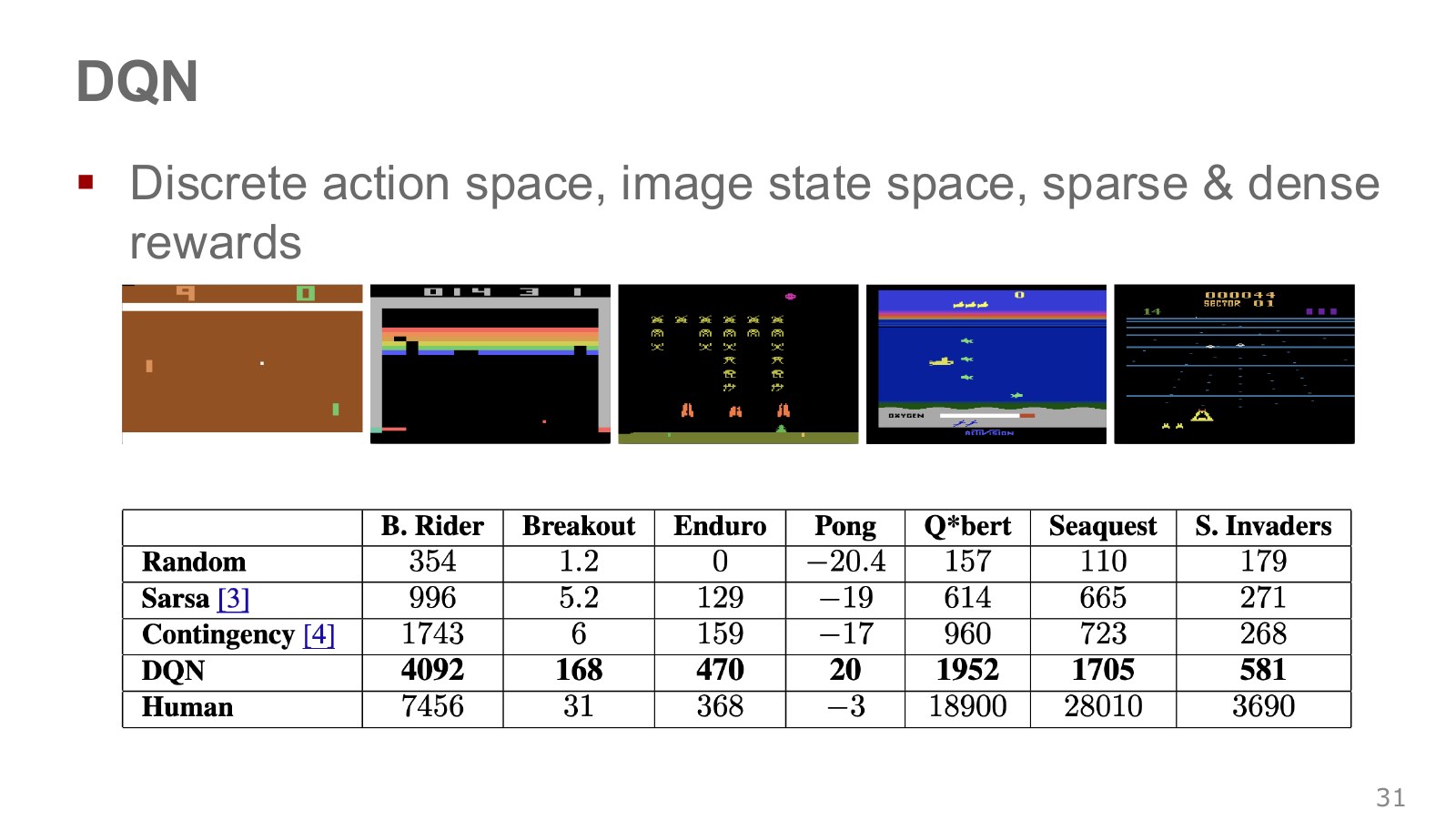
The screens above show distinct games supplying observations. Table columns are games; rows compare random policies, earlier methods, DQN and human performance. Each entry is that game’s score. Adding values across columns does not yield a universal intelligence score.
In the source table, DQN scores 168 versus human 31 on Breakout, but 1705 versus 28010 on Seaquest. Exceeding human score in one game does not establish the same result everywhere. Pong also includes negative scores, complicating simple score-ratio interpretations.
The table reports the seven-game 2013 results. A spoken 47 in the transcript or 49 elsewhere is not its column count. Generality here means applying a common architecture and learning method broadly instead of designing a separate specialized solution for each game.
#P033 · Why maximization can magnify estimation errors
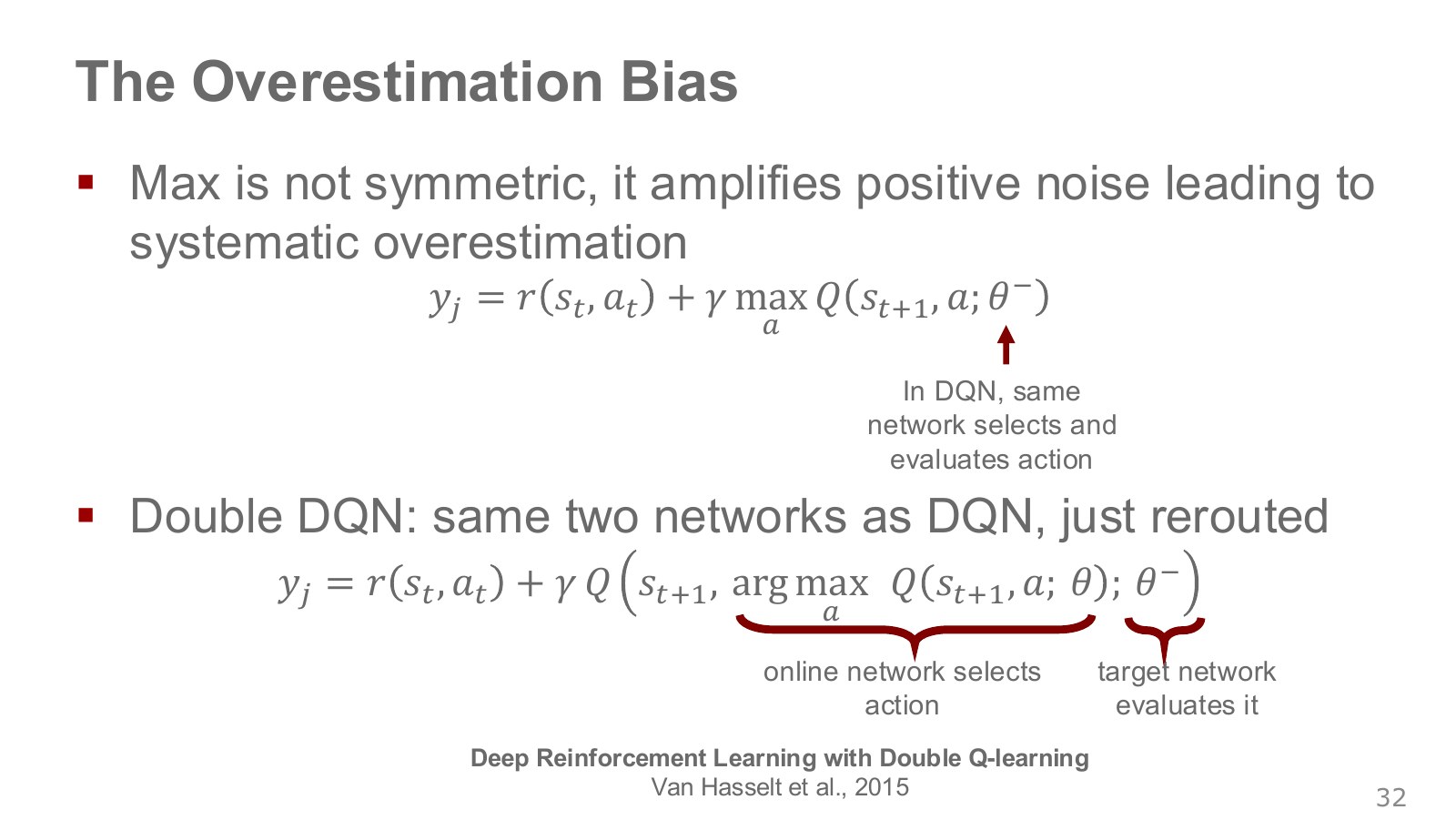
Two actions with equal true value can still have estimation errors. Selecting the larger estimate tends to favor one that happened to err upward. This is the intuition for overestimation bias.
For unbiased estimates of the same action values, in expectation the maximum estimate can be at least the maximum true value. This does not say that every individual maximum is too high: one sample may underestimate all actions.
Double DQN selects the next action with the current network and evaluates that action with the target network, reconnecting the two networks’ roles.
Explore the symbols and calculation Double DQN separates the network selecting an action from the network evaluating it
Read the equation in words
Separate the computation selecting a promising action from the computation evaluating that action. This aims to reduce the problem of directly reusing the maximum error in the same estimates.
Understand each symbol
- Action value estimated by a neural network with these weights. It is not guaranteed to equal the true value.
- The separate network's value estimate used to compute targets. The superscript minus denotes delayed weights, not a negative number.
- The reward received at one step: a learning signal defined so that larger is better.
- The discount factor for future rewards. Zero considers only the immediate reward, while values near one give more weight to the distant future.
- An indicator equal to 1 for actual termination and 0 otherwise. It prevents adding future value after termination.
- The next action selected by the current network.
- Select the input attaining the largest or smallest value, rather than the value itself.
Follow the calculation
- Use the current network to select the highest-valued action in the next state.
- The target network evaluates that specific selected action, rather than another action it prefers.
Check with a small example
With current-network values [5,4] and target-network values [2,6], select the first action and use its target evaluation, 2. Do not use the target network's maximum, 6.
An illustrative example for understanding the equation.
Suppose current-network outputs are 2 and 1, while target-network outputs are 0.5 and 1.5. Standard DQN takes target maximum 1.5. Double DQN instead evaluates the current network’s first-action choice using the target network, obtaining 0.5. The networks can remain correlated, so separation alone does not remove all bias or always yield a better policy.
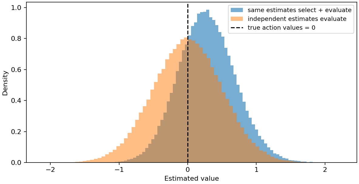
Original paper by van Hasselt et al..
#P034 · In continuous action spaces, we cannot enumerate every candidate
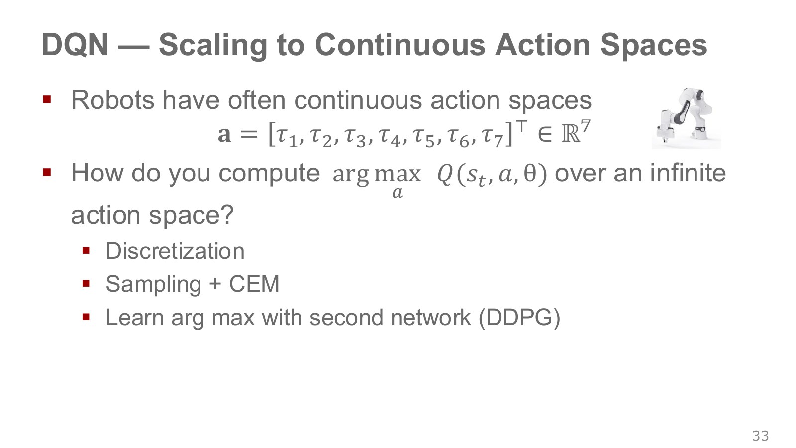
If we command a separate torque for each of a robot arm’s seven joints, the action is a vector of seven real numbers. We write it as , but real hardware imposes limits and units. A seven-dimensional action space is very different from a space containing seven possible actions.
Even discretizing each joint into just ten values produces combinations. Evaluating every combination with quickly becomes expensive as the dimension increases. A neural network may evaluate values quickly, but finding a good action still takes computation.
This chapter compares three approaches: use the geometry of the problem to discretize actions, sample candidates and search, or learn a separate policy that proposes the best action. This does not mean that continuous functions cannot be maximized. The difficulty is finding the maximum of a general nonlinear neural network quickly and accurately.
#P035 · Representing pushing and grasping through image positions and orientations
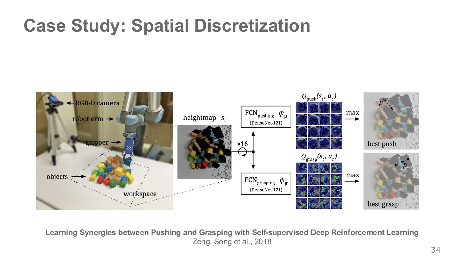
The RGB- camera on the left measures both color and depth. Converting its data into a top-down heightmap makes each pixel correspond to a position on the work surface and the height at that position. This differs from an ordinary perspective image, where equal pixel distances need not represent equal physical distances.
The two networks in the middle evaluate pushing and grasping separately. Rather than producing a single output, each fully convolutional network (FCN) produces a dense spatial map. A bright location means that starting the corresponding action there is expected to lead to a better outcome.
The ×16 label and multiple small maps indicate that sixteen orientations are considered. The original paper rotates the input heightmap in 22.5-degree increments and compares 32 maps in total: sixteen for pushing and sixteen for grasping. The final action combines action type, position, and orientation. The dot and line on the right indicate the selected action’s position and direction.
This method does not directly output every combination of torques for seven joints. People define the pushing and grasping action primitives and the workspace; inverse kinematics and motion planning handle lower-level execution. Learning determines when and where to choose those prepared actions. Zeng et al., original paper, pp. 3–4.
#P036 · What if a push helps a later grasp?
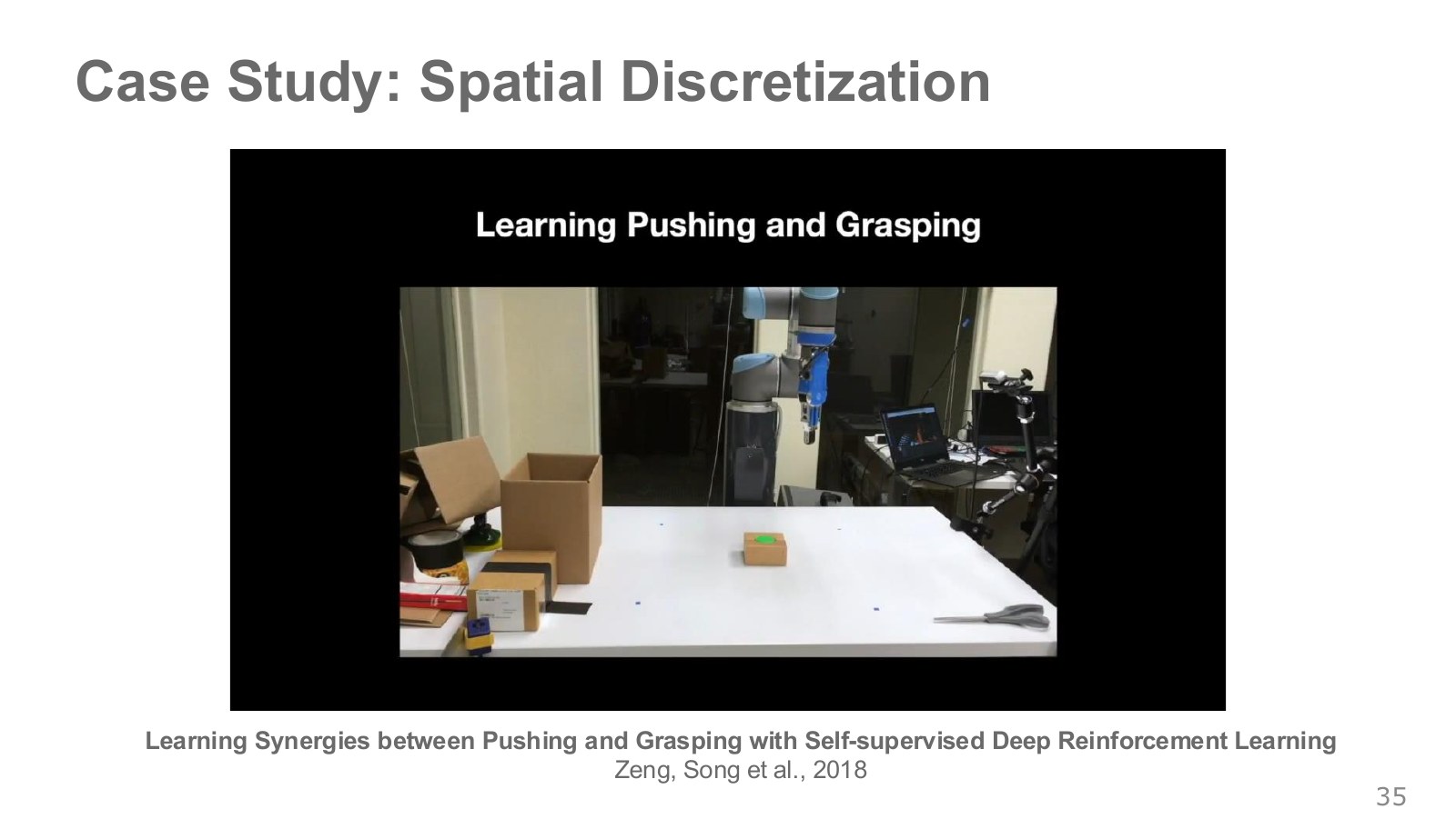
Objects packed together can be difficult to grasp immediately. Pushing one object aside first may make the subsequent grasp more likely to succeed. This is where long-term value matters: a push need not lift an object immediately to increase the grasping value of the next state.
The Bellman update passes the high grasping value of the separated state back to the preceding push. The pushing behavior in the video is a strategy learned from the reward, rather than a fixed execution sequence supplied by a person. Paper on the synergy between pushing and grasping
The Bellman update propagates the next state’s good value back to the earlier push. It can therefore account for the benefit of preparation, unlike a method that selects actions solely by immediate grasp success.
Do not read this as saying that everything emerged without any design. The original paper specifies the pushing and grasping actions, heightmaps, learning signals, and success criteria. Its reward assigns 1 to a successful grasp and 0.5 to a push that produces a detectable scene change. Describing the experiment as giving pushes no immediate reward would be inaccurate. What people did not prescribe was the exact sequence “push first, then grasp” for every scene. Methods in the original paper · Research project and code.
#P037 · Sampling and comparing candidate actions
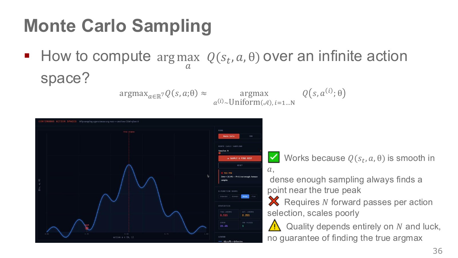
The simplest continuous optimization approach samples candidate actions within the valid range and compares their values. Here, Monte Carlo sampling simply means using random samples.
Explore the symbols and calculation Sampling returns the best action among the candidates actually drawn, rather than the best across the entire continuous space
Read the equation in words
When all continuous actions cannot be compared, sample a finite set of candidates and choose the best among them. Better actions outside that set can be missed.
Understand each symbol
- Action value: the average return obtained by taking a particular action in the current state and then following the policy.
- The action candidates actually sampled.
- The sampled candidate with the highest estimated value.
- Select the input attaining the largest or smallest value, rather than the value itself.
Follow the calculation
- Draw a finite set of candidates from the possible continuous actions.
- Score them with the critic and return the best candidate.
Check with a small example
If force candidates are only −1, 0, and 1, a true optimal force of 0.4 cannot be selected directly. Both the sampling method and the number of candidates matter.
An illustrative example for understanding the equation.
The high peak in the graph marks a region of actions with large values. To choose a good action, a candidate has to land near it. Smoothness of alone does not ensure that a finite random sample will contain an action near the global maximum. Narrow good regions and high dimensions make them easy to miss.
If a single sample has a 1% chance of entering a good region, 100 independent samples have about a 63.4% chance of entering it at least once. This simple example shows that even a fairly large sample can fail. The probability is calculated as .
With candidates, roughly evaluations of are needed. The candidates can, however, be processed in parallel as one minibatch; this does not necessarily mean waiting for sequential network calls. Berkeley’s discussion of continuous actions from 1:57 also explains this trade-off between accuracy and parallel computation.
#P038 · CEM: concentrating the next samples around good candidates
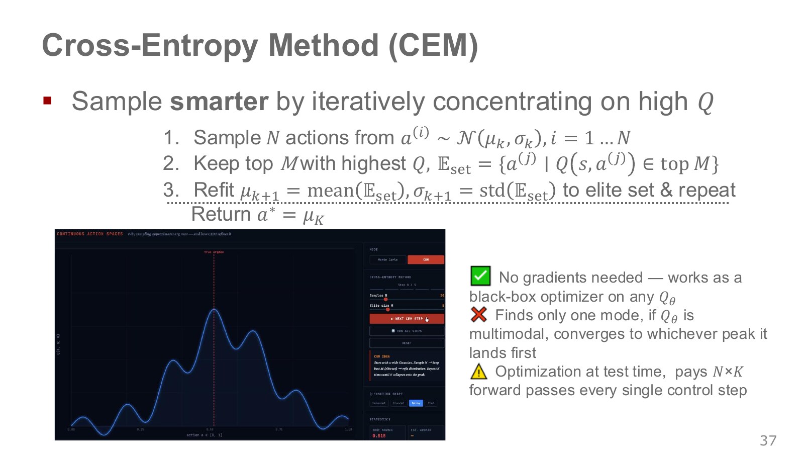
The Cross-Entropy Method (CEM) is an iterative optimization method that updates a candidate distribution. Instead of repeatedly sampling the entire range in the same way, it concentrates subsequent samples around candidates that scored well.
- Sample candidate actions from a distribution with the current mean and variance.
- Select an elite set of candidates with the highest values.
- Refit the distribution using those candidates’ mean and standard deviation.
- Repeat for a fixed number of iterations and return an action.
In the original figure, and describe the center and spread of the current candidate distribution. They do not represent uncertainty about the environment’s state or the policy’s probability of success. Exploration may stop if the variance approaches zero too quickly, so a lower bound can help. Samples must also respect the actual action limits.
This single-Gaussian version may collapse onto one of several peaks or concentrate incorrectly between them. CEM need not always use this particular distribution, but this simple version offers no global-optimality guarantee. With candidates and iterations, action selection costs roughly evaluations of .
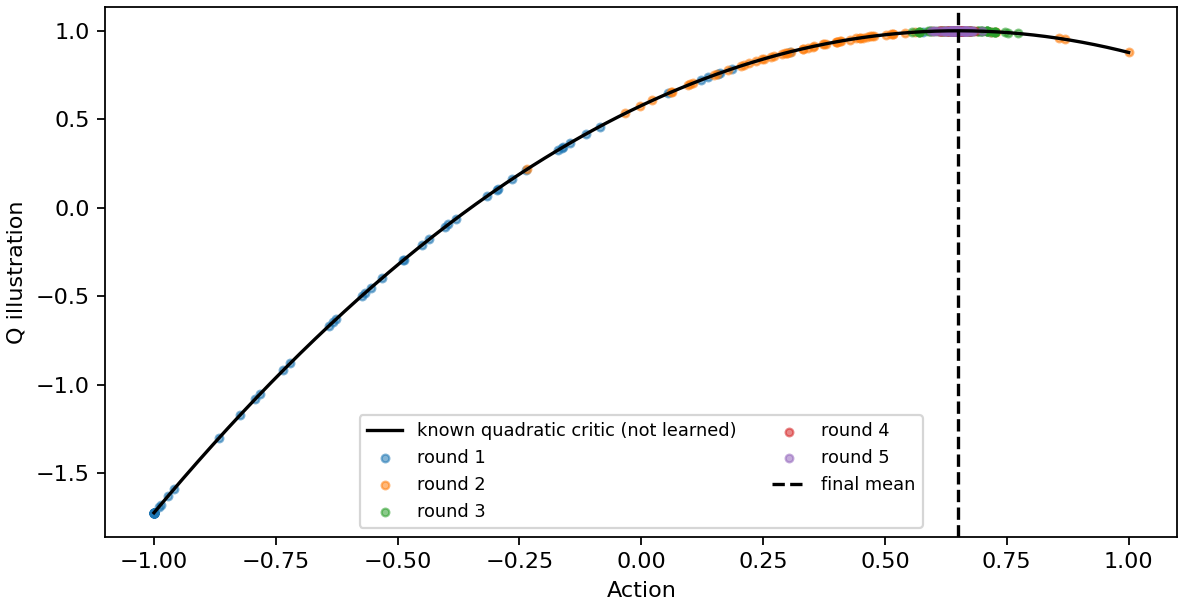
Berkeley’s CEM explanation from 3:21.
#P039 · QT-Opt: searching for actions while reusing real robot data
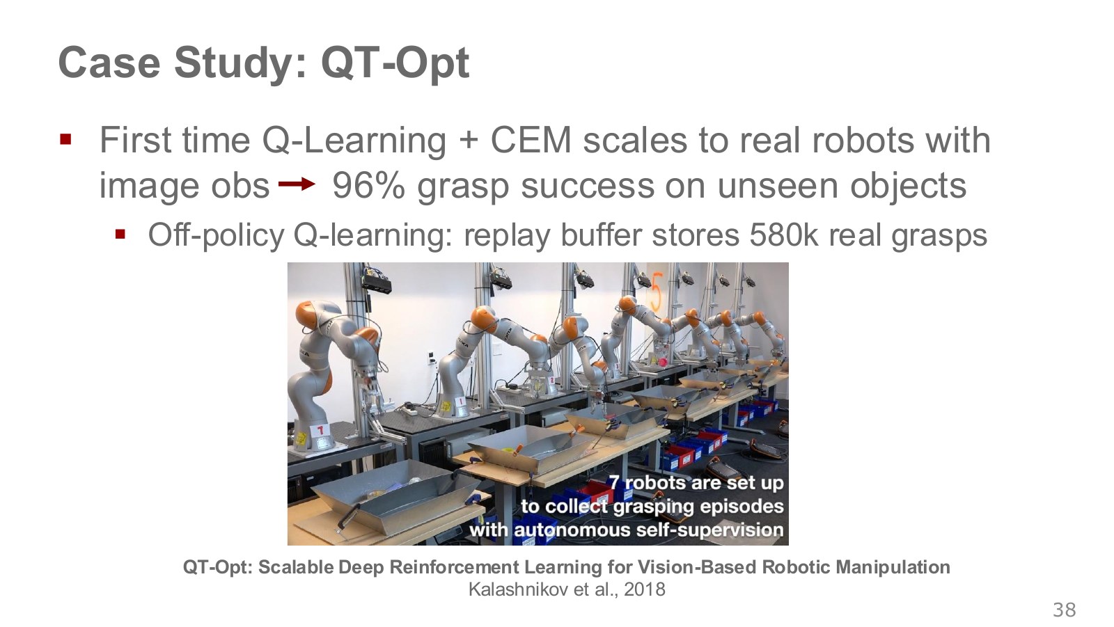
The robots in the photograph collect different grasping experiences. QT-Opt applies an image-conditioned function and CEM-based continuous action search to a large real-world dataset. Reusing expensive robot transitions multiple times through a replay buffer is an important part of this approach.
The original paper reports more than 580,000 real-world grasp attempts and a 96% grasp success rate in its evaluation on unseen objects. This does not mean that the training set contained 580,000 photographs, or that every robot achieves 96% success on every object and task. It is an experimental result with specified objects, equipment, and evaluation procedures.
Rather than choosing a grasp point from a single initial image and executing the entire action unchanged, the method uses closed-loop control to adjust its grasping strategy in response to observations during execution. Regrasping or moving an object through contact can be understood as actions that improve the eventual grasp outcome. We should not turn this into a broad historical claim such as “the first real-world Q-learning.” Original paper by Kalashnikov et al..
#P040 · DDPG: learning the action search itself with a neural network
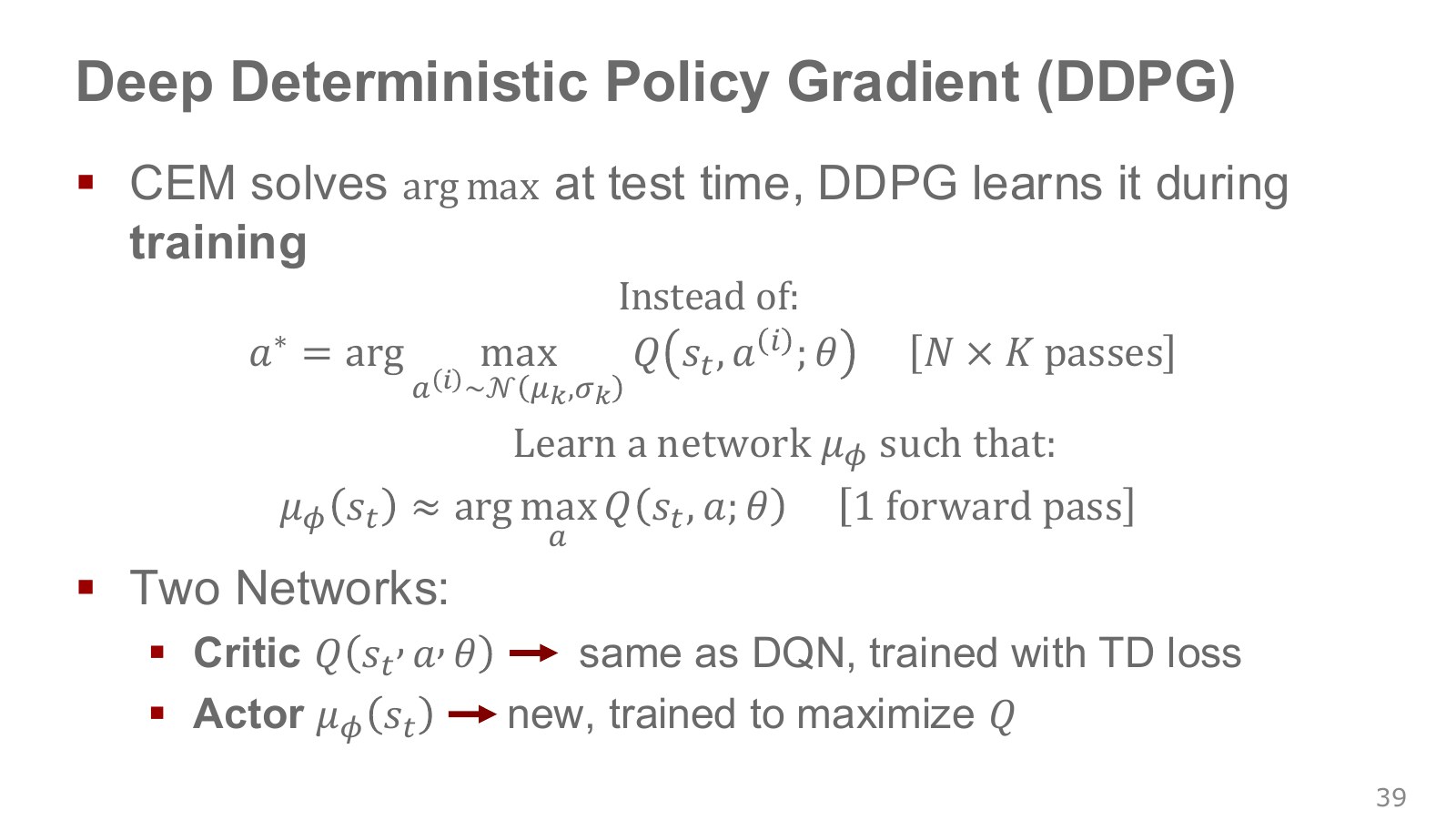
CEM compares candidates again each time the robot acts. Deep Deterministic Policy Gradient (DDPG) instead learns a network that directly outputs a good continuous action from a state. This network is the actor. The network that evaluates actions is the critic.
Explore the symbols and calculation The actor directly outputs an action from the state, and the critic evaluates that action's long-term value
Read the equation in words
Instead of searching the critic for a good action every time, learn an actor that directly produces a good action from the state.
Understand each symbol
- A deterministic actor that takes a state and directly outputs a continuous action.
- Action value estimated by a neural network with these weights. It is not guaranteed to equal the true value.
- Weights of a different network. Read which model they belong to together with the calculation steps.
- The parameters collecting the trainable weights of the network or policy.
- Select the input attaining the largest or smallest value, rather than the value itself.
Follow the calculation
- The actor outputs a continuous action for the current state.
- The critic evaluates the action, and the actor is improved to obtain higher value.
Check with a small example
Instead of comparing 1,000 action candidates for each state, one actor pass can output force 0.4. Whether it is truly optimal depends on the critic's accuracy.
An illustrative example for understanding the equation.
Here, denotes the actor’s weights and the critic’s weights. For the same state, the actor proposes a command and the critic estimates how good it is. The actor moves toward commands the critic values more highly, while the critic learns from a TD target based on the reward and next state.
The original slide’s “two networks” refers to these two roles. A practical DDPG implementation also has target copies of both, so there are more than two network instances. A typical critic target takes the following form.
Explore the symbols and calculation DDPG constructs its target by evaluating the next state's target-actor action with the target critic
Read the equation in words
The target critic evaluates the action the target actor would produce in the next state to construct DDPG's training target. The maximum over all continuous actions is not computed directly.
Understand each symbol
- The reward received at one step: a learning signal defined so that larger is better.
- The discount factor for future rewards. Zero considers only the immediate reward, while values near one give more weight to the distant future.
- An indicator equal to 1 for actual termination and 0 otherwise. It prevents adding future value after termination.
- The target actor and target critic, whose weights are updated with a delay.
Follow the calculation
- Pass the next state through the delayed actor to obtain an action.
- Evaluate that action with the delayed critic, discount the result, and add the immediate reward.
Check with a small example
If the next actor action is evaluated at 6, reward is 1, and the discount factor is 0.9, the target is 6.4. On actual termination, it is 1.
An illustrative example for understanding the equation.
At deployment, one forward pass through the actor can propose an action. The symbol indicates an approximation; it does not prove that the actor finds the true global maximum in every state. Berkeley’s introduction of the actor and target copies, 6:15–9:42.
#P041 · The actor gradient connects derivatives through the critic and the actor
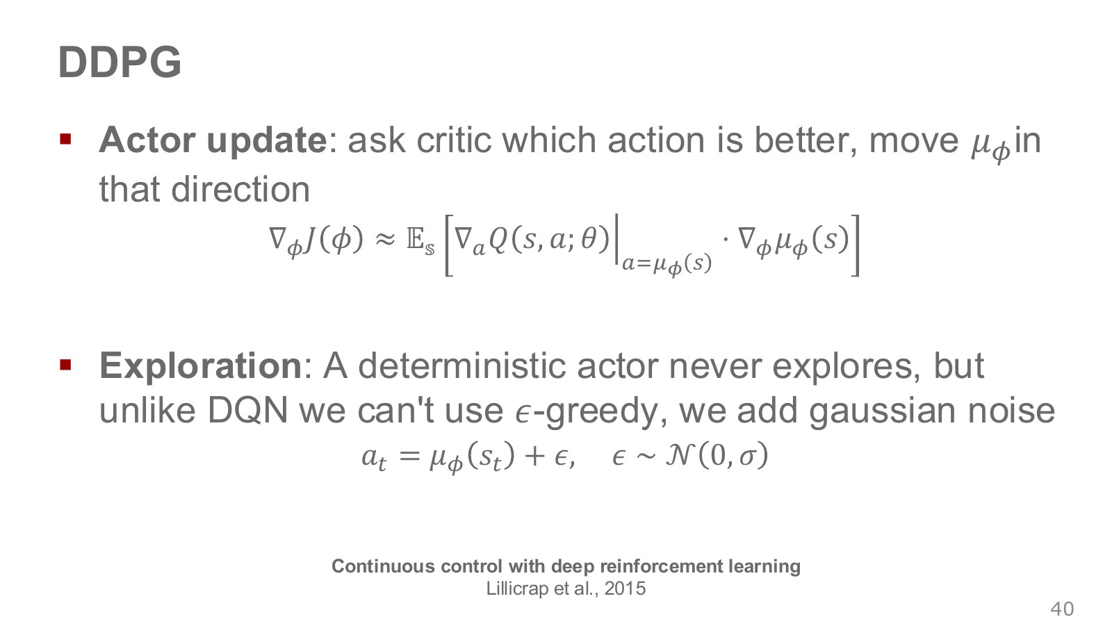
If the critic indicates that moving the action slightly in a particular direction increases , we adjust the actor’s weights in that direction. The chain rule connects the sensitivities of these two changes.
Explore the symbols and calculation The actor update uses the chain rule to connect changes in value with respect to the action to changes in the action with respect to the weights
Read the equation in words
Multiply how value changes with a small action change by how the action changes with a weight change. This is the chain rule for differentiating a composite function.
Understand each symbol
- A deterministic actor that takes a state and directly outputs a continuous action.
- Action value estimated by a neural network with these weights. It is not guaranteed to equal the true value.
- Weights of a different network. Read which model they belong to together with the calculation steps.
- The parameters collecting the trainable weights of the network or policy.
- The direction and rate at which value changes as the action changes.
- The rate at which the output action changes as the actor weights change.
- An expectation: an average over possible outcomes weighted by their probabilities.
- A gradient collects componentwise derivatives describing how much the result changes when a variable changes.
Follow the calculation
- Compute the critic's action gradient at the current actor action.
- Connect it with the actor's weight derivatives and update the actor in the direction of increasing value.
Check with a small example
In one dimension, if the value derivative with respect to the action is 2 and the action derivative with respect to the weight is 3, the value derivative with respect to the weight is .
An illustrative example for understanding the equation.
The term describes how the score changes when the action changes, while describes how the action changes when the weights change. For vectors, the calculation uses the appropriate Jacobian product. Computing the actor-loss gradient does not mean updating the critic’s own weights together with the actor.
In the article’s one-dimensional example, , , , and give a current action of 0.4. The derivative with respect to the action is 0.5, and the derivative of the action with respect to the weight is 2, yielding a product of 1. The executable example also checks this against a finite difference obtained by slightly changing the weight.
A deterministic actor returns the same action for the same input, so data collection often adds noise to its actions. Randomly mixing in actions probabilistically is not mathematically impossible in a continuous space; local noise is simply a common alternative. Action limits and noise magnitude must be specified, and adding independent Gaussian noise does not automatically produce temporally smooth commands.
The original DDPG paper used temporally correlated Ornstein–Uhlenbeck noise. The Gaussian-noise diagram in the original lecture should be read as a simplified explanation of exploration.
#P042 · Fast action output does not solve training stability
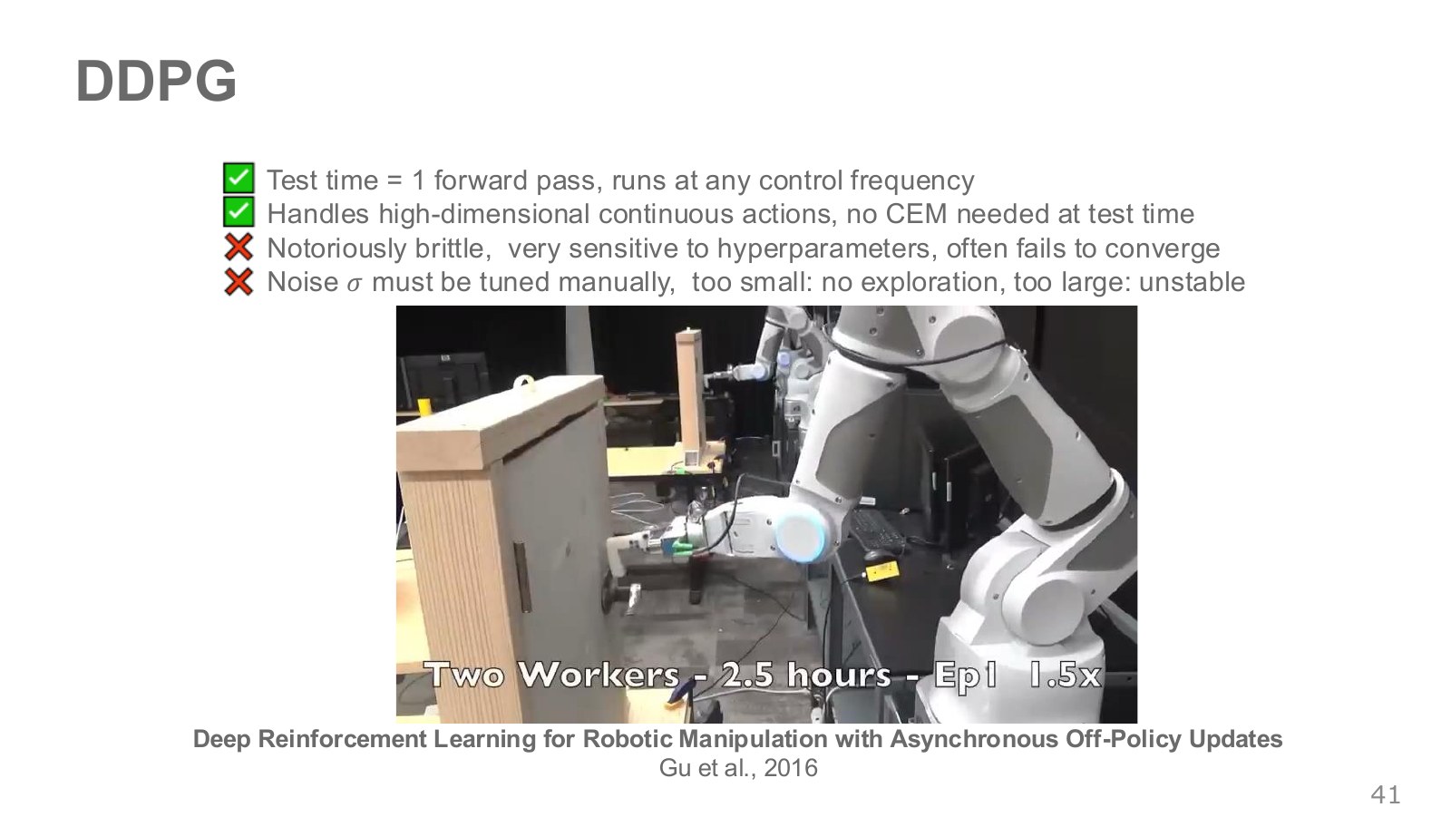
The photograph of a robot manipulating a door or handle illustrates an application to continuous control. An actor removes the need to run a CEM candidate search at every step. It does not mean that the system always runs at any control frequency. The entire latency must be measured, including model size, image processing, hardware, and communication.
For exploration, the illustrated DDPG setup adds small Gaussian noise to the actor’s continuous commands. This makes it easy to try actions near a normal approach trajectory. If the noise is too small, other routes are rarely visited; if it is too large, commands fluctuate substantially during training.
DDPG can be sensitive to critic error, the actor’s exploitation of that error, exploration range, and learning rate. If the actor actively seeks actions the critic overvalues, predicted can rise even as actual returns fall.
Labels such as “two workers, 2.5 hours” in the original video describe a particular research experiment. They are not universal specifications promising that your robot will learn in the same time. Gu et al.’s asynchronous off-policy robot learning is a real-world research example, separate from the calculations performed for this article.
#P043 · Choosing a method means considering the model, state, actions, and learning conditions together
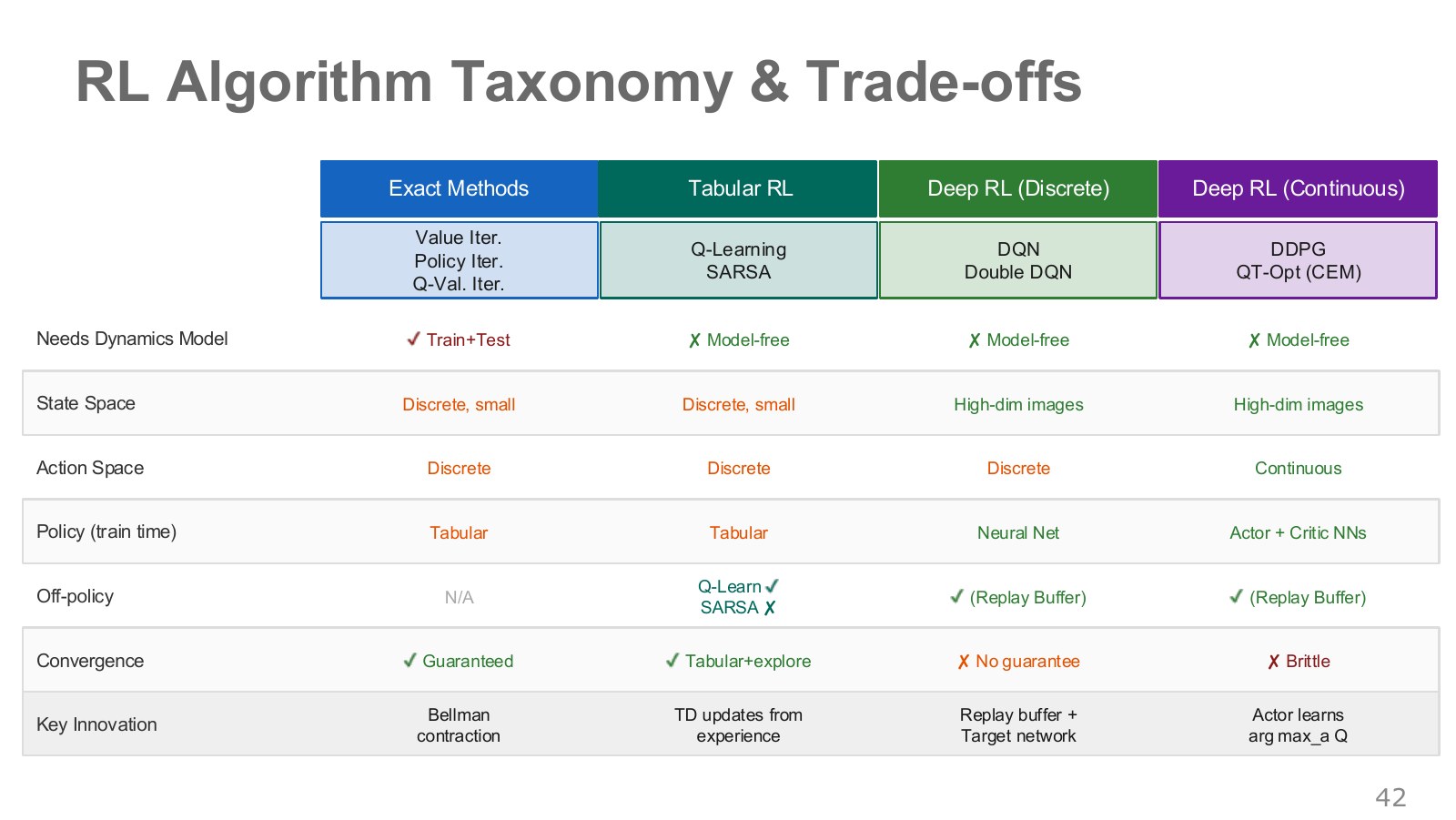
The table’s columns cover the four groups discussed in this chapter: computing tables from a known model, learning tables from experience, learning discrete-action values with neural networks, and handling continuous actions.
| Question | Tabular dynamic programming | Tabular Q-learning and SARSA | DQN and Double DQN | QT-Opt and DDPG |
|---|---|---|---|---|
| Is the transition model used directly? | Yes | Sampled experience | Sampled experience | Sampled experience |
| How is the state represented? | Small state table | Small state–action table | Neural features, images, etc. | Neural features, images or vectors, etc. |
| How are actions selected? | Model-based improvement or a stored policy table | Compare the table | Compare outputs for finite actions | Candidate search or an actor |
| Can old experience be reused? | Computation uses the model itself | Yes for Q-learning; SARSA requires attention to policy consistency | Replay | Off-policy replay |
| Key conditions for guarantees | Finite discounted MDP, exact computation, etc. | Conditions on visits, learning rates, and policy changes | No general global-convergence guarantee | No general global-convergence guarantee |
Do not memorize the original table as a strict set of mutually exclusive categories. value iteration can use a model during learning yet execute using the stored . Within the continuous-action column, QT-Opt still pays a search cost, unlike DDPG’s direct actor output. Images are not a requirement either: DQN can also handle continuous-vector states with discrete actions.
Even methods described as “model-free” differ in their data requirements, execution time, and action representations. For a robot problem, ask together whether the model is known, whether observations contain the necessary information, whether actions can be enumerated, and how much expensive experience can be collected.
#Calculations run and checked for this article
The article computes value iteration and policy iteration in a small 3×4 stochastic grid, then runs tabular Q-learning on 240,000 sampled transitions. Entering the goal or hazard gives +1 or −1 and terminates the episode; the discount factor is 0.9. All other immediate rewards are zero. This is a separate environment with explicitly defined walls, boundaries, and slipping, rather than a reproduction of the ETH demo or assignment.
Q-learning uses individual next states and rewards sampled by the simulator, rather than an expected target from a precomputed transition matrix. Valid state–action pairs are queried uniformly to control visitation coverage. This experiment therefore does not compare sample efficiency for learning through exploration from the start of each episode.
Eighteen checks cover transition-probability sums, avoiding duplicate terminal rewards, Bellman fixed points, exact policy evaluation, agreement between value and policy iteration, nondecreasing improvement, state–action coverage, learned error, the learned policy’s value gap, TD calculations, terminal targets, Double DQN’s separation of selection and evaluation, noisy-maximum bias, CEM, and the actor’s chain-rule derivative. In this run, the maximum estimation error was about 0.0269, and the learned greedy policy matched the optimal policy’s value within numerical tolerance in this small environment. Settings, seeds, and all numerical results are recorded with the executable code and JSON/CSV results.
These are not training results for DQN or DDPG neural networks or a real robot. The CEM example searches a predefined quadratic function, and the noise experiment involving two estimators is also distinct from an actual Double DQN experiment.
#Continuing with the official assignment
The official ETH HW4 connects these concepts to executable implementations. This article refers to the instructions and relevant files at a pinned commit; it does not claim to have implemented and run the official assignment on the reader’s behalf.
| Assignment section | Questions to connect with this chapter |
|---|---|
| Ex1: value and policy iteration in GridWorld | Do both methods produce the same policy under the same model? How does the route change as slipping becomes more likely? |
| Ex2: CartPole DQN | Have you distinguished four continuous state variables from two discrete actions? What are the replay-buffer and target-network update intervals? |
| Ex3 and Ex4: PPO and SAC on SO100 | How do the policy and data-reuse strategy change for continuous actions? These algorithms connect to later chapters. |
Seeing CartPole in the original assignment does not mean that its algorithm directly outputs robot joint torques. The SO100 assignments also use normalized joint-position commands, so distinguish their physical meaning from this chapter’s illustrative torque vector.
Chapter 05 continues with methods that improve policies directly and explores continuous control further.
#Sources and further reading
- ETH Robot Learning, Lecture 4 · Video · PDF · Image copies
- David Silver — Dynamic Programming · Lecture video · Model-Free Control · Lecture video
- Berkeley CS285: Value Functions · Deep RL with Q-Functions · Target-network video · Continuous-action video
- DQN 2013 · DQN 2015 · Double DQN
- Pushing and grasping · QT-Opt · DDPG · Asynchronous real-world robot learning
P numbers follow the file order of the image copies. Slides devoted solely to acknowledgments or references are omitted. Copyright in the slides belongs to Oier Mees and the respective rights holders of included material. Diagrams from the original DQN paper belong to their original authors. The grid, noise, and CEM figures are separate educational calculations created for this article.