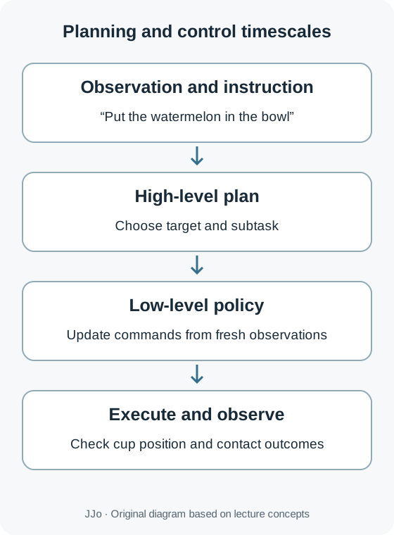
Reinforcement Learning 10 — When Should a Robot Think Longer?

Tell a robot, “Put the watermelon slice in the bowl.” If a watermelon-shaped toy sits beside real watermelon, the robot must identify the target before reaching. But when a grasped slice starts slipping, there is no time to wait for a long explanation. This chapter examines separating time spent deciding what to do from the control cycle executing it. Previous chapter: Generalist Robot Policies

This is week ten on ETH’s official schedule; the lecturer calls it Lecture 11 in the recording. The Korean transcript was compared with English captions. P numbers below follow the copied slides, including the cover, and slides can be opened through links. ETH schedule · Official PDF · Slide-copy index

Two timescales for planning and control. Observation/instruction → high-level plan → low-level policy → actual execution/observation. — Two timescales for planning and controlJJo; original conceptual diagram · Original source

#What more demonstrations give a robot

#P002 · Is scaling data enough?

More demonstrations teach a robot which actions are common in particular scenes. These expectations form prior knowledge. But locating a target on an unfamiliar table or recombining steps to grasp a handle requires connecting known objects and movements to the current scene. The lecture’s embodied reasoning grounds plans in actual views, end-effector positions, and object interactions. Original lecture, 0:20 · Slide P002

#P003 · The missing ability: recombining knowledge for new problems

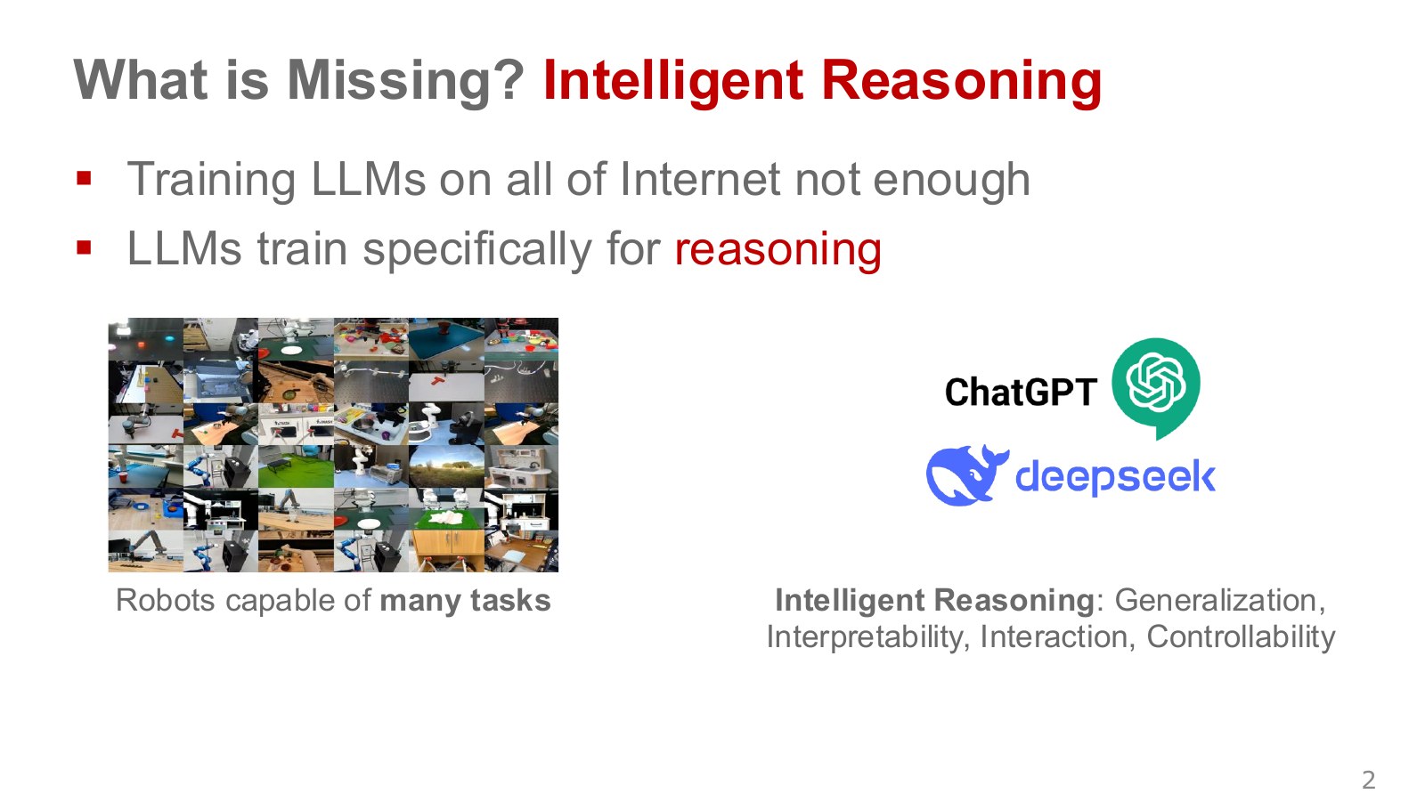
Demonstration learning compresses frequently chosen human actions into model weights. Yet even a familiar instruction such as “put it in the right bowl” needs reconsideration if that bowl is inverted or the target occluded. Compositional reasoning reconnects known objects, spatial relationships, and action orders. It does not promise to solve every unseen situation; it asks whether existing knowledge can help without demonstrating each situation in full.

#P004 · Can reasoning join a multimodal sequence?

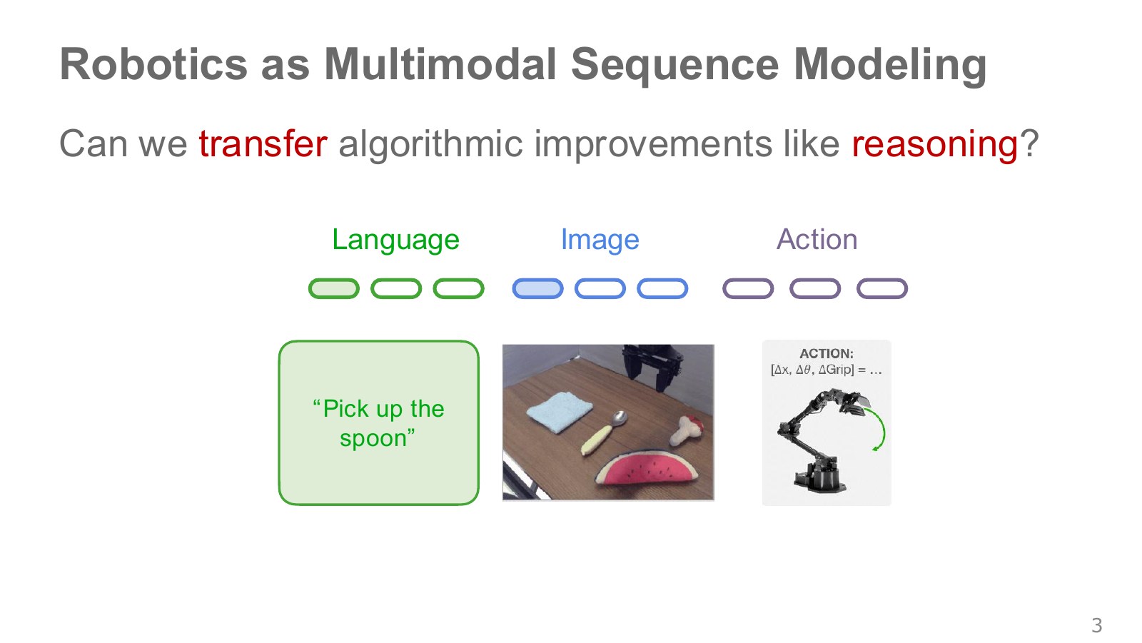
Chapters 7–9 connected images, language, and actions within model sequences, creating a point of contact with LLM reasoning improvements. Plausible verbal plans alone are insufficient. The plan’s “watermelon” must refer to a particular camera-visible object, and its approach must correspond to a physical hand path.

#What does ECoT write before acting?

#P005 · Acting through plans, subtasks, and screen locations

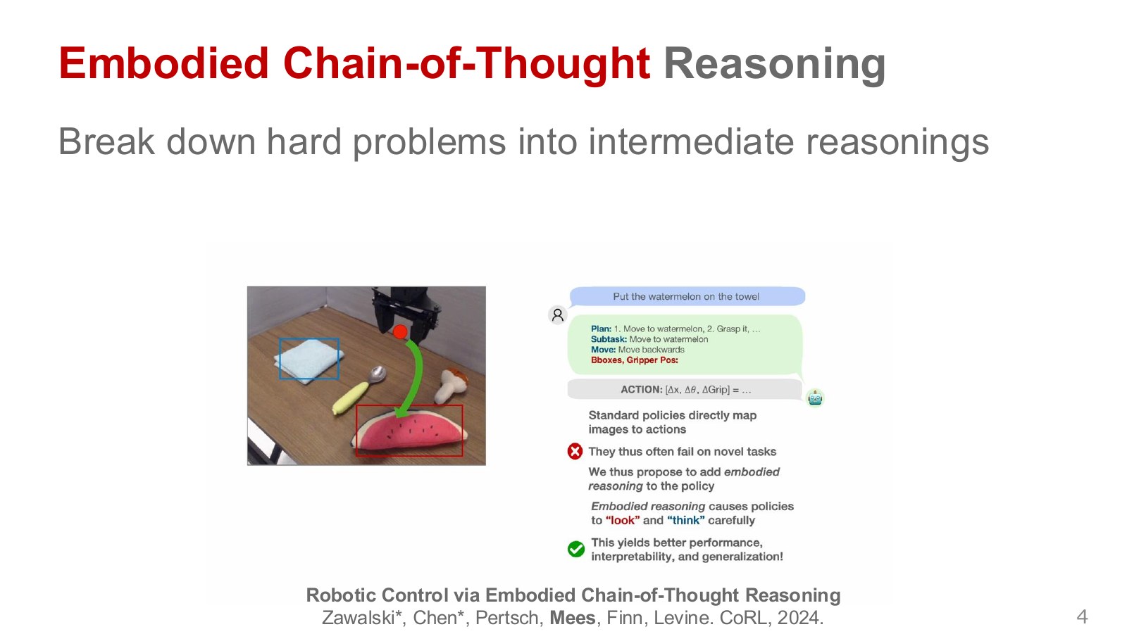
Embodied Chain-of-Thought (ECoT) makes a vision–language–action model output intermediate plans and observations before predicting motor commands. For the watermelon example, it produces a subtask such as moving toward the slice, the target’s bounding box, current gripper position, and movement direction. The plan narrows the goal, and the box locates it on screen. Original lecture, 5:16 · Slide P005 · ECoT paper

#P006 · Adding reasoning annotations to existing trajectories

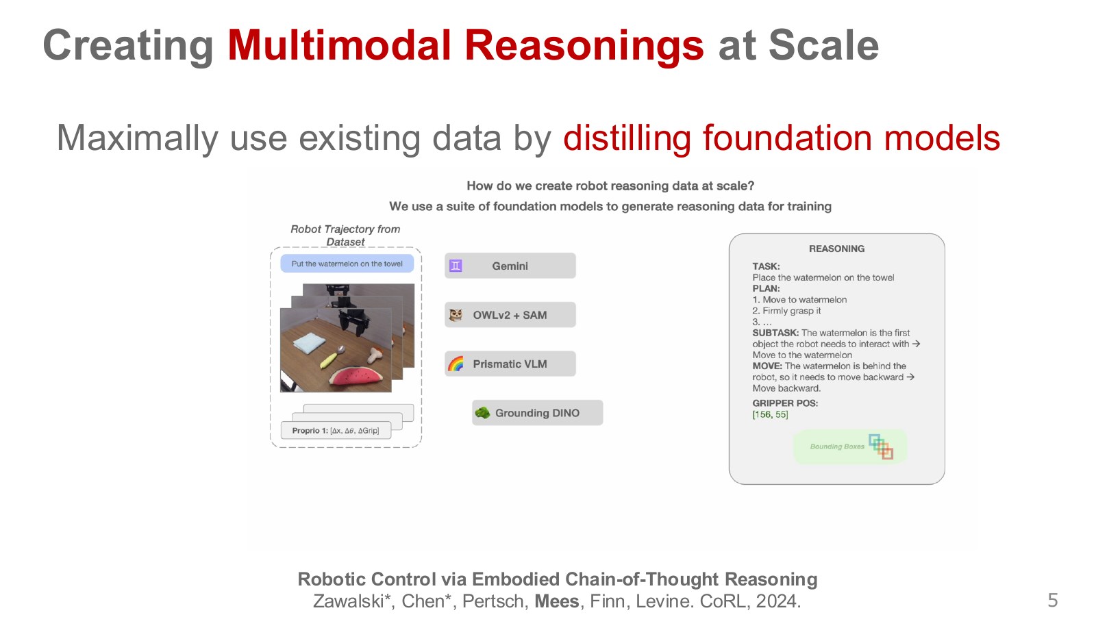
Existing demonstrations contain images and actions, but people do not annotate plans and boxes at every instant. The researchers add reasoning annotations using pretrained models and trajectory-derived position and motion information. In simplified form, one policy call’s joint reasoning-and-action probability factors as follows.

#P007 · Generating actions conditioned on reasoning tokens

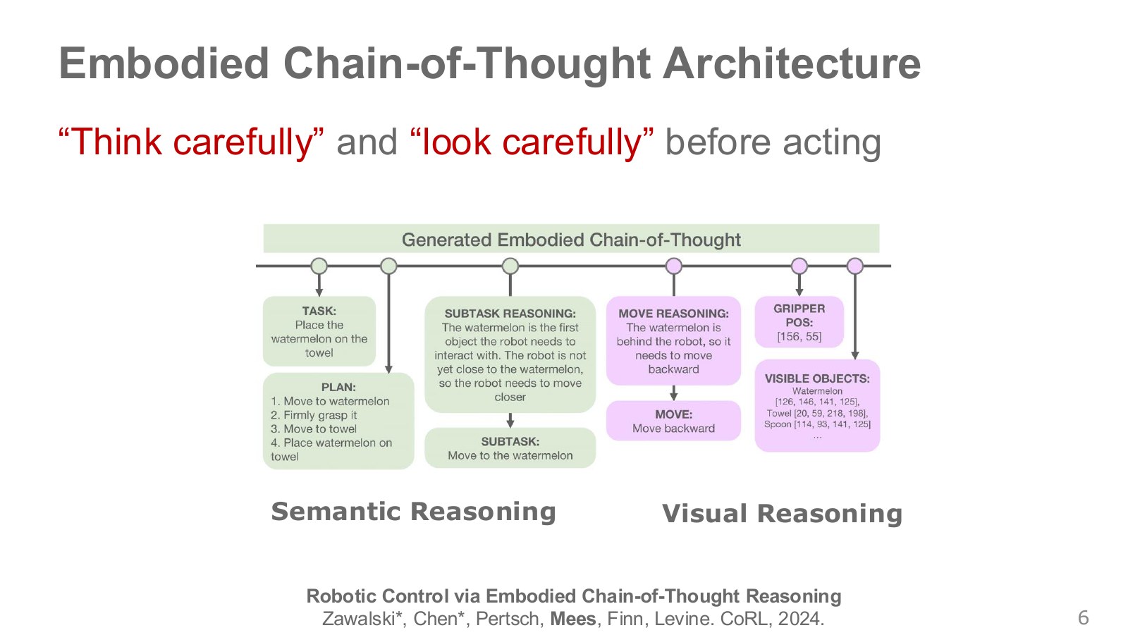
Distinguish annotation generation from deployment prediction. Training attaches plans, subtasks, object boxes, gripper information, and movement descriptions to existing demonstrations to form target sequences. The model predicts these intermediates from observations and instructions, then reads them to predict action tokens. Deployment does not supply future ground-truth trajectories. Automatic annotations can contain errors, so location and movement annotation quality affects action learning.

p_\theta(r,a\mid o,g)=p_\theta(r\mid o,g)\,p_\theta(a\mid o,g,r)

Explore the symbols and calculation Factoring reasoning and action into two conditional probabilities

Read the equation in words

For the same scene and goal, first generate an intermediate judgment, then choose an action with that judgment added to the input.

Understand each symbol

$o$: The current observation, such as a camera image.
$g$: An instruction or goal specifying the object.
$r$: Intermediate tokens containing plans, bounding boxes, and similar information.
$a$: The action corresponding to a hand-motion command.
$p_\theta$: Probability determined by the policy weights.

Follow the calculation

Hold observation and goal fixed and read the probability of an intermediate judgment.
Read the action probability conditioned on that judgment too, then multiply the two.

Check with a small example

If identifying the watermelon as the target has probability 0.8 and selecting a correct move afterward has probability 0.75, their joint probability is 0.60.

An illustrative example for understanding the equation.

#P008 · Evaluation on new objects, instructions, and spatial relationships

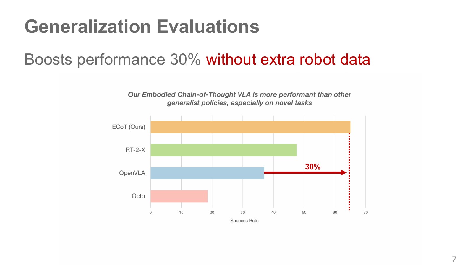
The paper reports a 28-percentage-point success-rate gain over baseline OpenVLA on evaluations with new instructions, objects, and spatial relationships—the difference rounded to about thirty in the lecture. It adds synthetic annotations to existing demonstrations without recording extra robot demonstrations for the comparison. The 7B ECoT model’s reported advantage over 55B RT-2-X also belongs to that evaluation scope. Original lecture, 8:05 · Slide P008 · ECoT paper

#P009 · People can edit intermediate plans

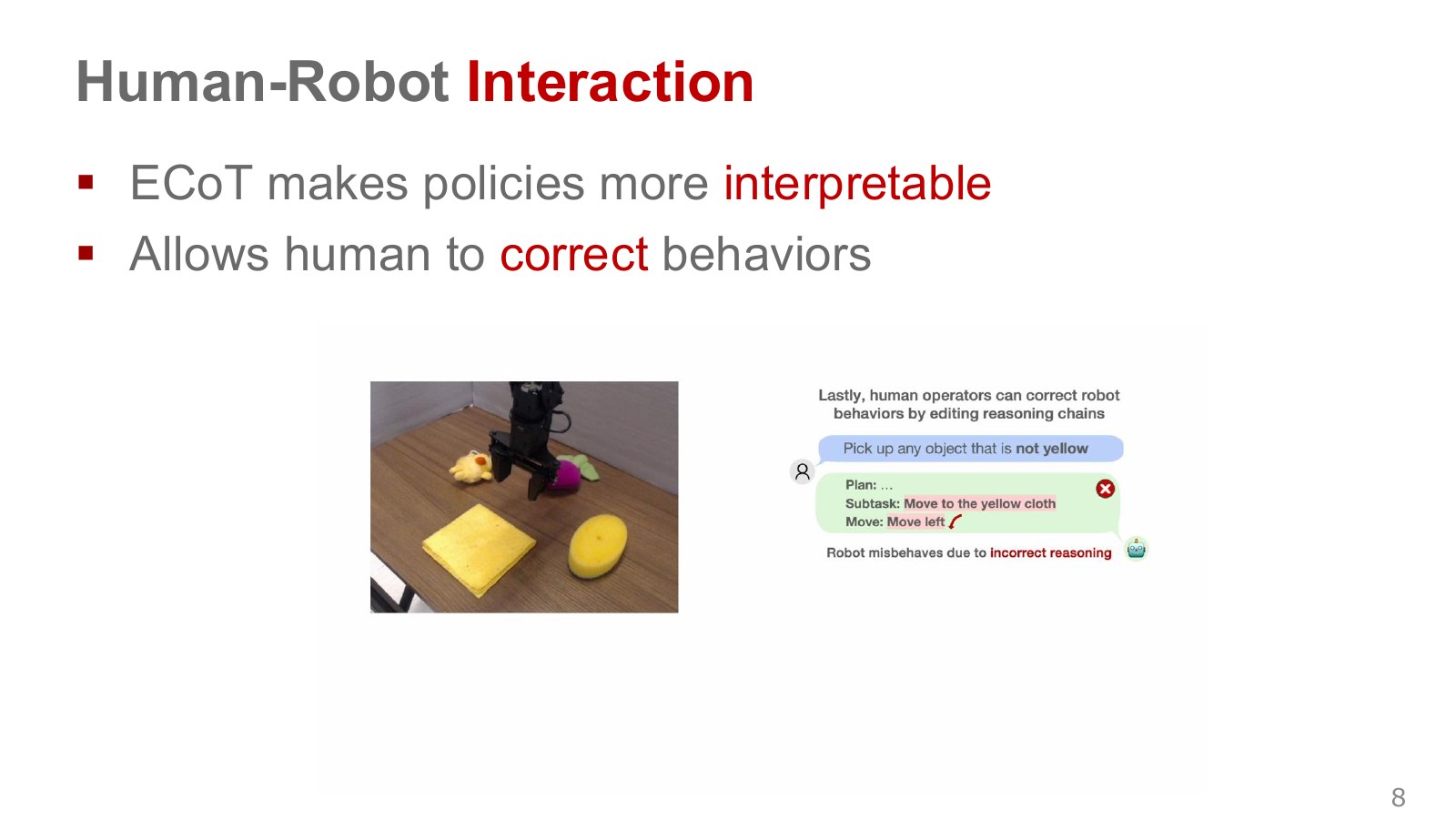
If a model boxes the wrong object, a person can correct the plan before execution. A model trained on reasoning annotations only from WidowX generated plausible reasoning on other robots and cameras, demonstrating transfer of intermediate representations. Validating actions on a new robot still requires manipulation evaluations there. MolmoAct’s depth tokens and editable end-effector paths provide another example of more directly spatial reasoning. Original lecture, 9:14 · Slide P009 · Slide P010 · MolmoAct paper

#P010 · Interpreting reasoning generated for new robots

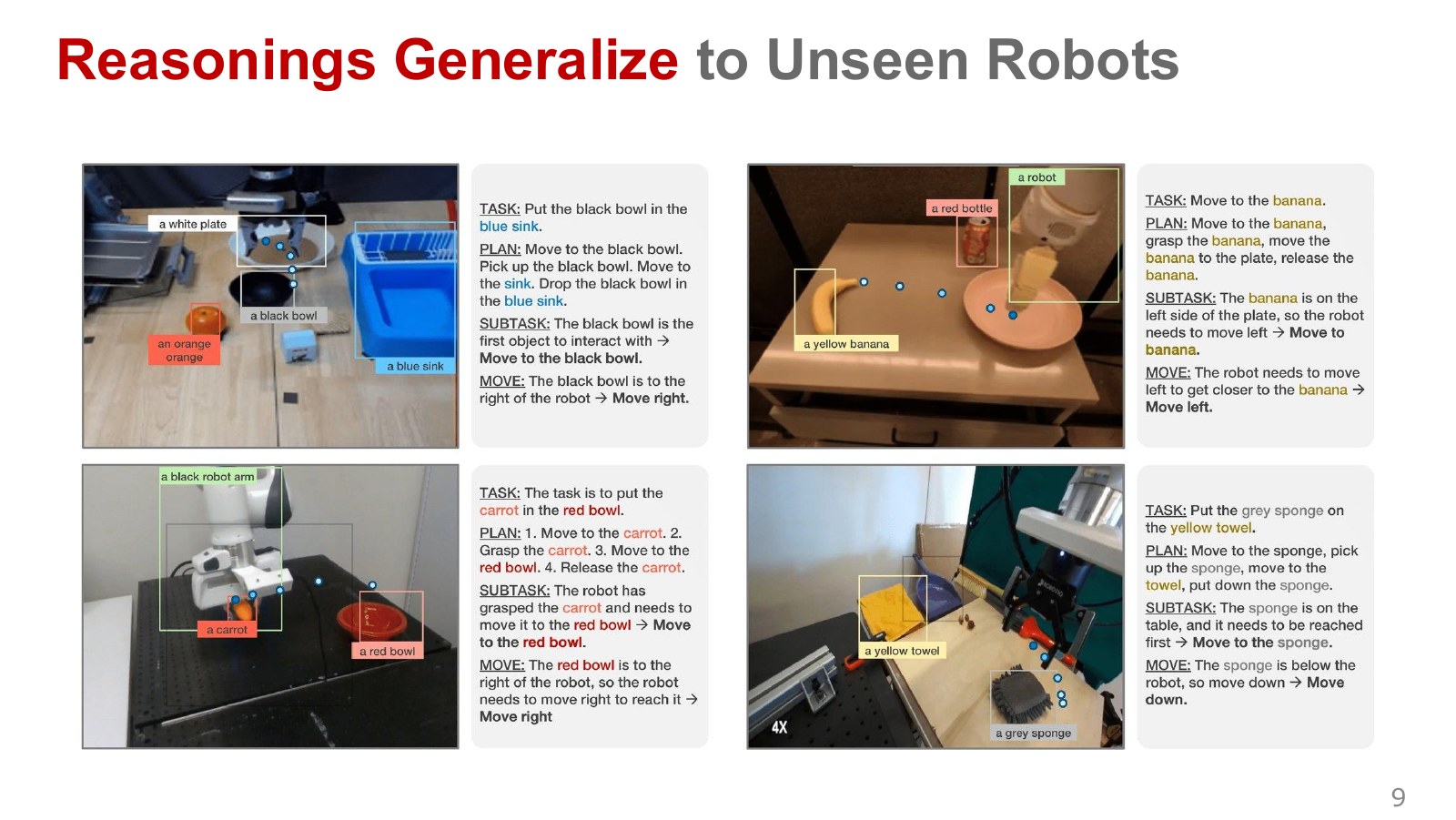
The reasoning annotations in this experiment came from WidowX data. Generating descriptions of targets and grippers in other OXE robot videos suggests that visual–language pretraining can help with new cameras and bodies. Transfer of descriptions, coordinate-estimation accuracy, and successful physical control remain separate evaluation targets.

#P011 · Reasoning as a policy-training objective

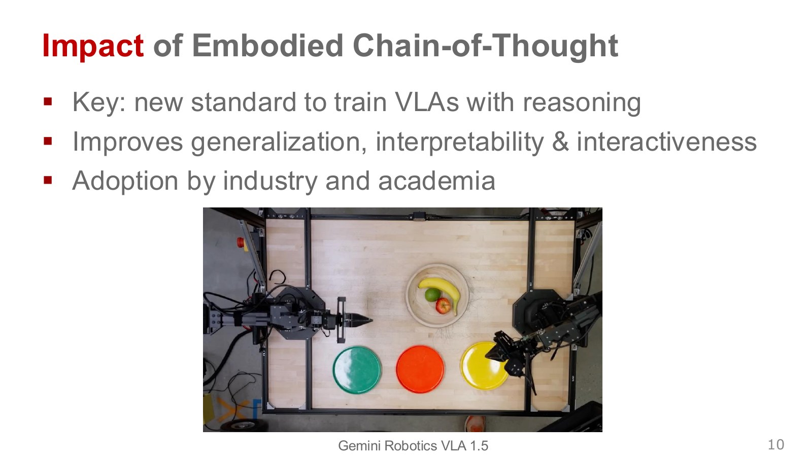
The lecturer describes later academic and industry models explicitly incorporating reasoning before actions. The key is treating reasoning as more than attractive text added to a display. Which reasoning targets are learned and how they enter action prediction become policy-design decisions. This does not imply full disclosure of every commercial model’s internals.

#P012 · Extending to depth, action-free human data, and visual plans

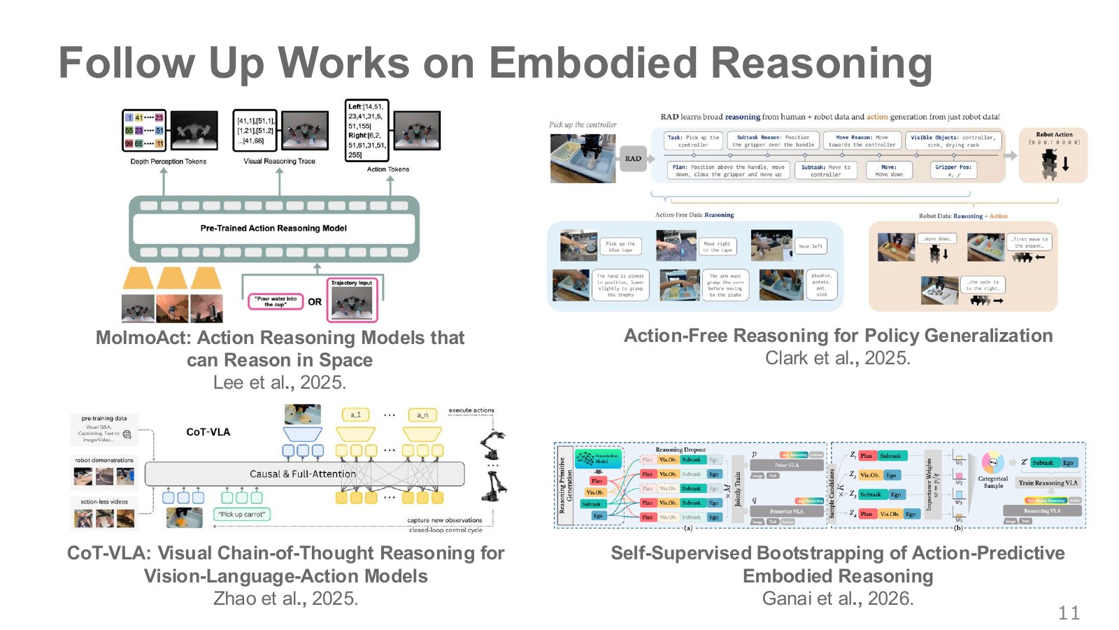
MolmoAct explores depth-grounded spatial reasoning; Clark and colleagues separate reasoning learning from action learning to use sources such as human data without robot action values. The slides also show CoT-VLA’s visual future plans and later work generating reasoning useful for action prediction. Compare whether reasoning consists of sentences, depth, points, or future images, and where action annotations are required.

#Intermediate representations people can correct

A correct subplan to approach watermelon can still place its box on the adjacent toy. Correcting only the target box tests whether subsequent actions change. Conversely, a correct box with a forward-push plan when the hand should withdraw calls for correcting movement. ECoT’s interaction interface helps isolate where an error begins.

The same distinction applies to plausible reasoning on new-robot videos. Language knowledge about objects and spatial relations may transfer across cameras and arms, but reachable ranges and allowed gripper poses differ. Evaluate intermediate explanation accuracy and final manipulation success separately. ECoT paper

#Latency revealed by the first WidowX rollout

#P013 · How different are 4 Hz and four seconds per action?

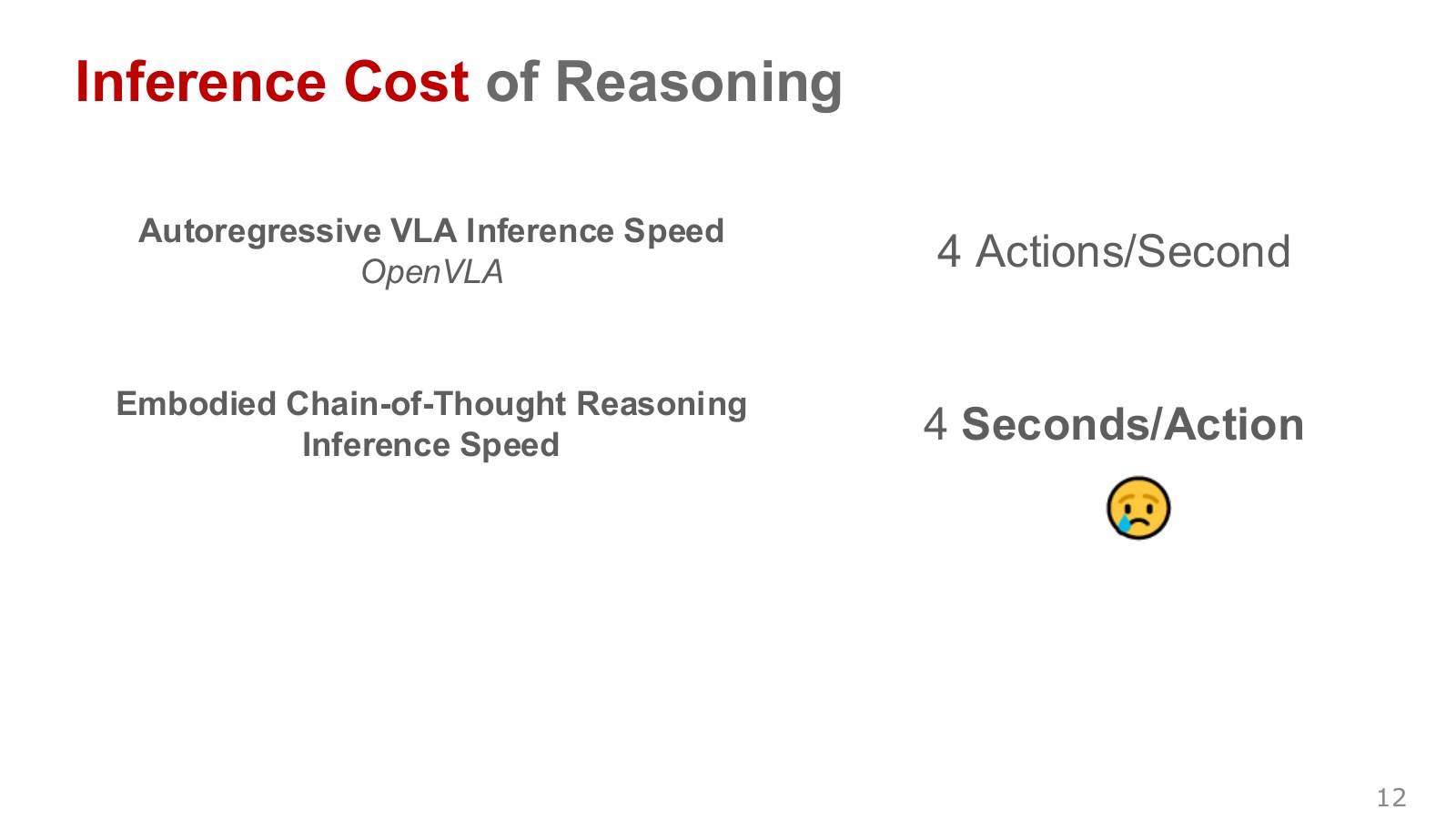
In the example setup, the slides compare basic OpenVLA at about four actions per second with full ECoT at one action every four seconds. Mees recalls how tedious it was to wait through a task when the team first deployed it on WidowX. These correspond to action intervals of 0.25 and 4 seconds. Camera-transfer and motor-control times need separate measurement. Original lecture, 13:49 · Slide P013

\Delta t=\frac{1}{f}

Explore the symbols and calculation Converting action-output frequency to a time interval

Read the equation in words

If actions are emitted one at a time at regular intervals, the reciprocal of outputs per second gives the interval per action.

Understand each symbol

$\Delta t$: The interval between action outputs, in seconds.
$f$: Actions emitted per second, in hertz.

Follow the calculation

Read the output count per second.
Divide one second by that count to obtain the time per action.

Check with a small example

Four actions per second means one every $1/4=0.25$ seconds. One every four seconds is 0.25 Hz. This simple comparison gives a sixteenfold interval difference.

An illustrative example for understanding the equation.

#P014 · Can reasoning benefits survive lower generation cost?

Those figures imply a sixteenfold difference between policy calls. An object moving little within 0.25 seconds may leave the anticipated hand position within four seconds. This compares policy inference in that experiment. Internal motor PID frequency and policy target-update frequency are separate, so low-level control can continue beneath a slow policy. The question is how frequently targets incorporate a fresh scene.

#Where did reasoning help?

#P015 · Testing three hypotheses for the benefit

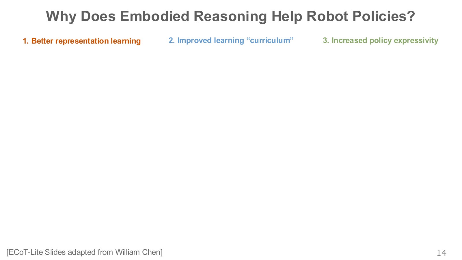
ECoT-Lite separates three possibilities: learning useful representations such as object positions, providing an intermediate learning scaffold between pixels and actions, or adding computational workspace irrespective of token meaning. In LIBERO-90 simulation, reasoning pretraining or occasional reasoning omission approached full ECoT’s performance. Meaningless-token variants showed no benefit. Evidence supports both learning useful representations and reading that information during action prediction. Original lecture, 15:49 · Slide P015 · Slide P019 · ECoT-Lite paper

#P016 · Hypothesis 1: better representations during training

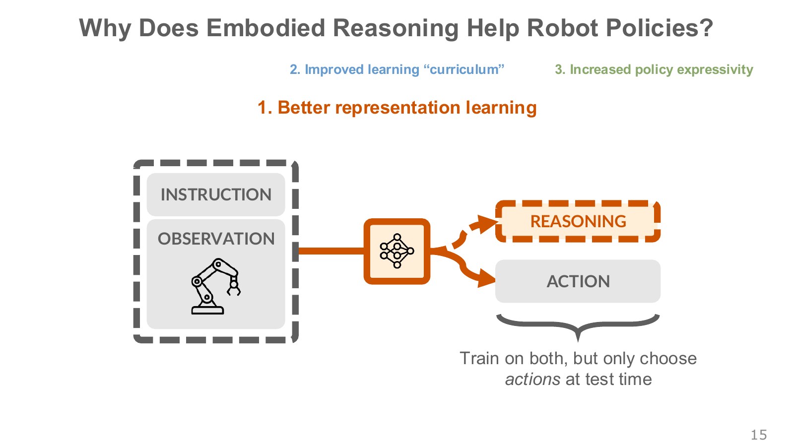
Reasoning annotations may teach action-relevant visual features such as an important handle. If this explains most gains, weights trained to generate reasoning should retain benefits when execution predicts only actions. This separates time spent printing reasoning from representations learned while training on it.

#P017 · Hypothesis 2: scaffolding difficult action prediction

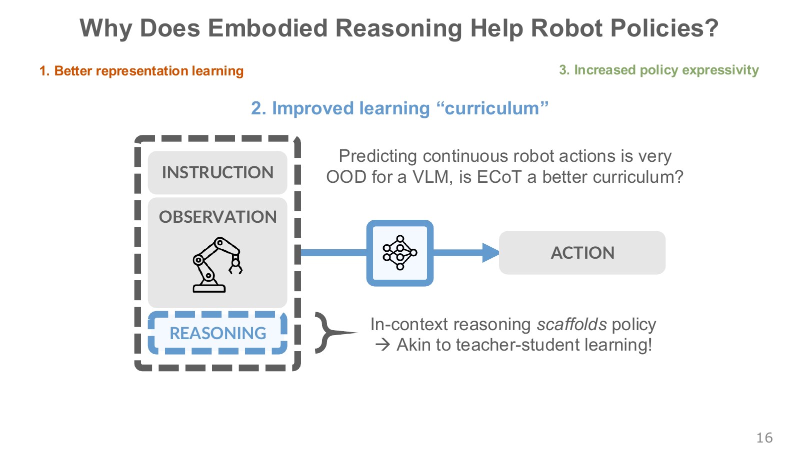
A VLM’s pretrained task of describing images differs substantially from outputting joint targets. Intermediate movement descriptions can break the pixel-to-action mapping into smaller connections. Scaffolding experiments supply reasoning as input without a loss for predicting it, separating extra supervision from the benefit of an input scaffold.

#P018 · Hypothesis 3: can meaningless tokens add workspace?

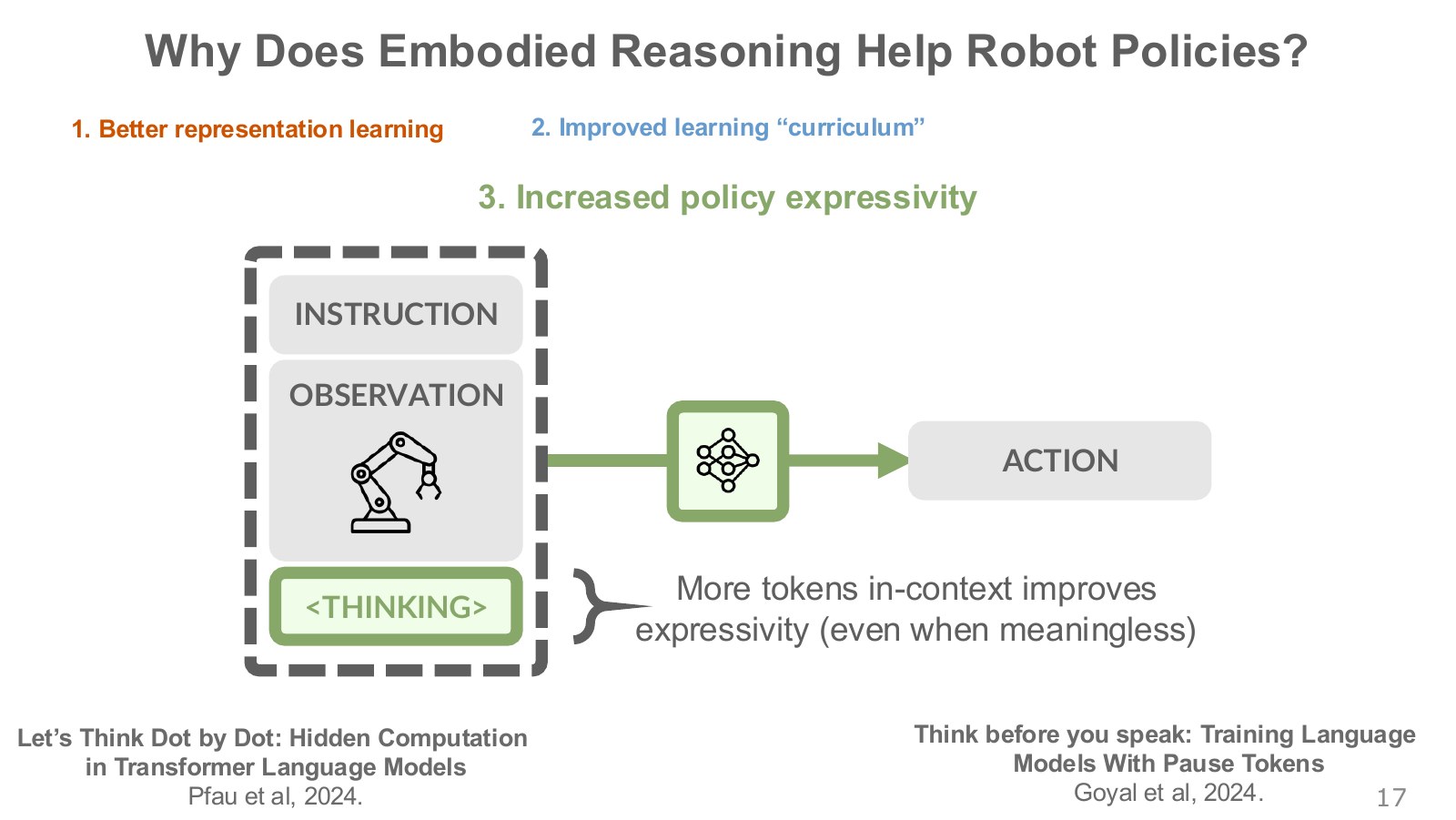
An autoregressive model reprocesses preceding context when generating another token. Even meaningless intermediate symbols could therefore provide sequential workspace. This tests useful reasoning content separately from increased computation. A phenomenon possible in language models does not automatically yield the same robot-policy benefits.

#P019 · What remained in the LIBERO-90 ablations?

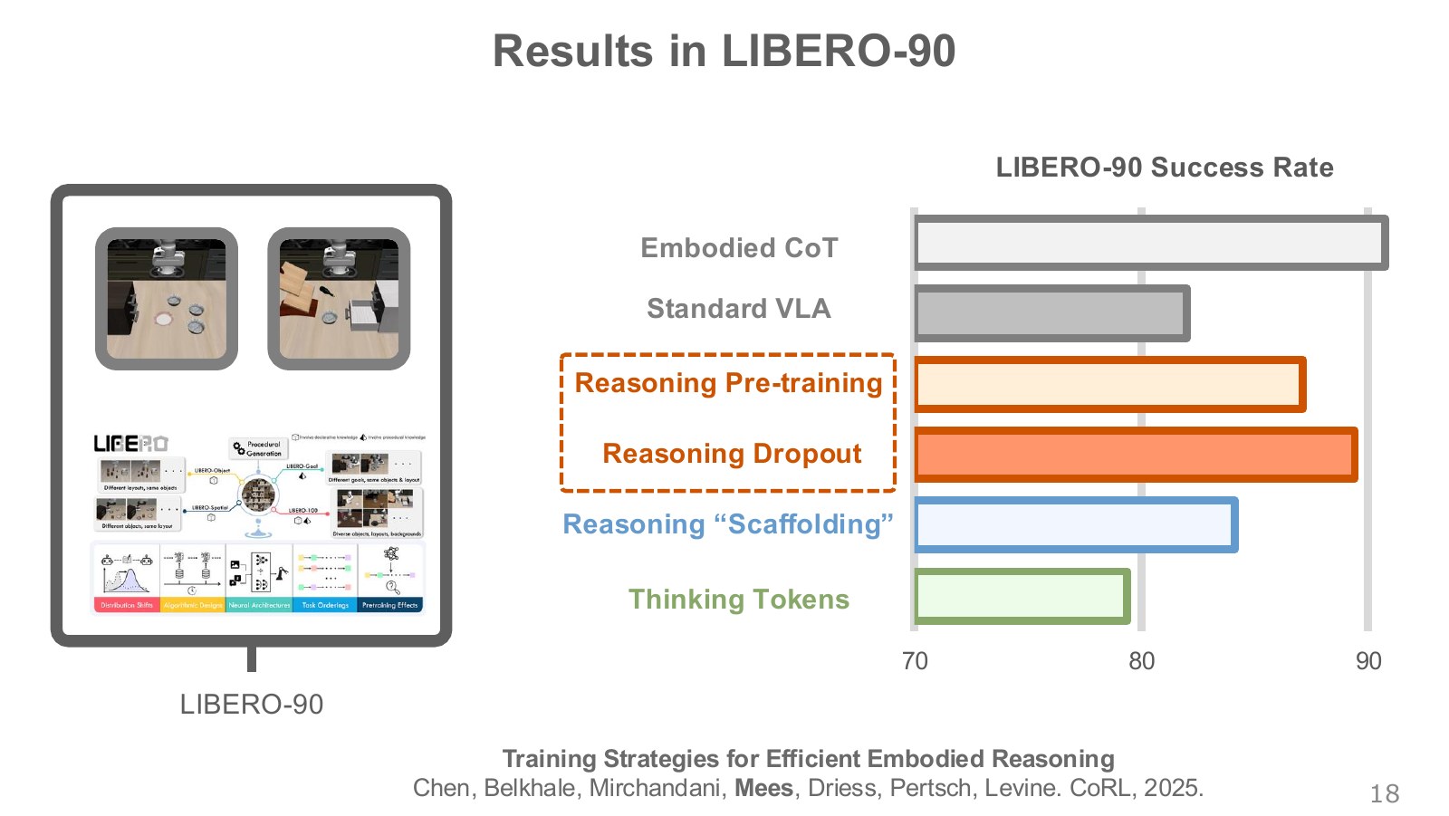
Reasoning pretraining and dropout approached full ECoT even when full reasoning was omitted during execution. Supplying reasoning as an input scaffold also helped. Meaningless thinking tokens did not improve baseline VLA in this setting, making extra token computation alone an insufficient explanation. No single experiment establishes one universal mechanism for all models.

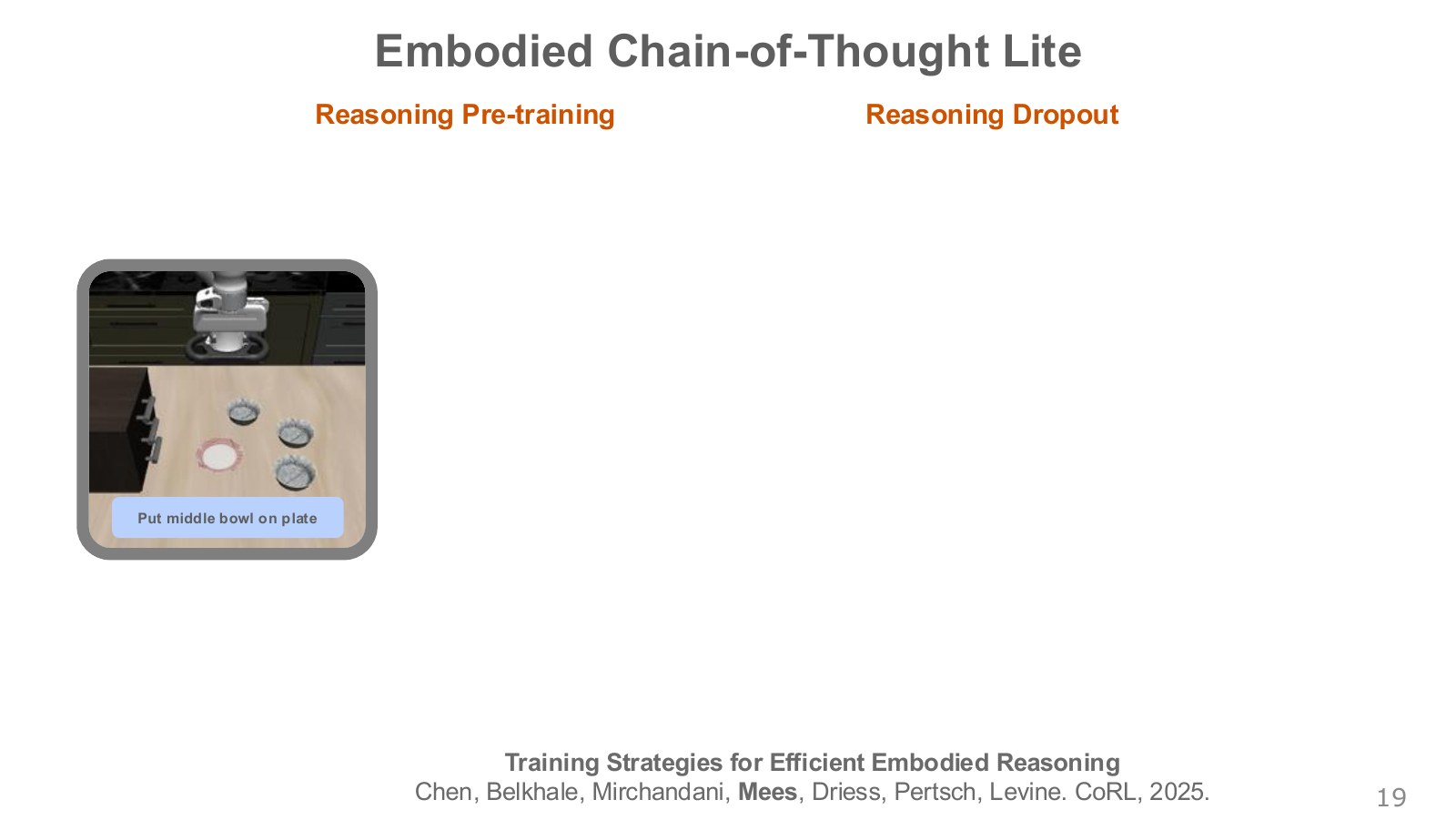
#P020 · ECoT-Lite: paths retained during training and execution

Training method	At deployment	Selection criterion presented in the lecture
Full ECoT	Generate intermediate reasoning, then actions	Human inspection or correction of explanations
Reasoning pretraining	Transfer reasoning-trained weights and output actions directly	Reasoning and action datasets are unpaired
Reasoning dropout	Omit reasoning probabilistically during training, enabling both deployment paths	Extended deliberation is needed only for unfamiliar scenes

The paper reports ECoT-Lite inference approximately three times faster than a standard reasoning policy. The earlier four-actions-per-second versus one-action-per-four-seconds example is a different comparison; do not combine those factors. Original lecture, 22:18 · Slide P020 · Slide P034 · Slide P035 · ECoT-Lite paper

#Computational order in reasoning pretraining and dropout

Reasoning pretraining first trains a VLM to explain object positions and plans. A second stage starts from those weights and predicts actual actions. Features learned in the first stage initialize action learning. This can connect human videos with reasoning annotations to separate robot data with action values.

Dropout jointly trains reasoning and actions while omitting reasoning for some examples. The model practices both reading reasoning context and acting directly from observations. Slides P020–P033 animate which inputs and losses remain in these methods. Holding the image and goal fixed while toggling reasoning tokens lets us compare action outputs and runtime. Slides P020–P033 · ECoT-Lite paper

Rather than reducing the three hypotheses to one claim, compare information in training losses with information read during action prediction. Reasoning supervision helped representations, and pathways using them also mattered. Meaningless-token results make pure computation increase an insufficient explanation on this benchmark.

#P033 · P020–P033: final states of the two training paths

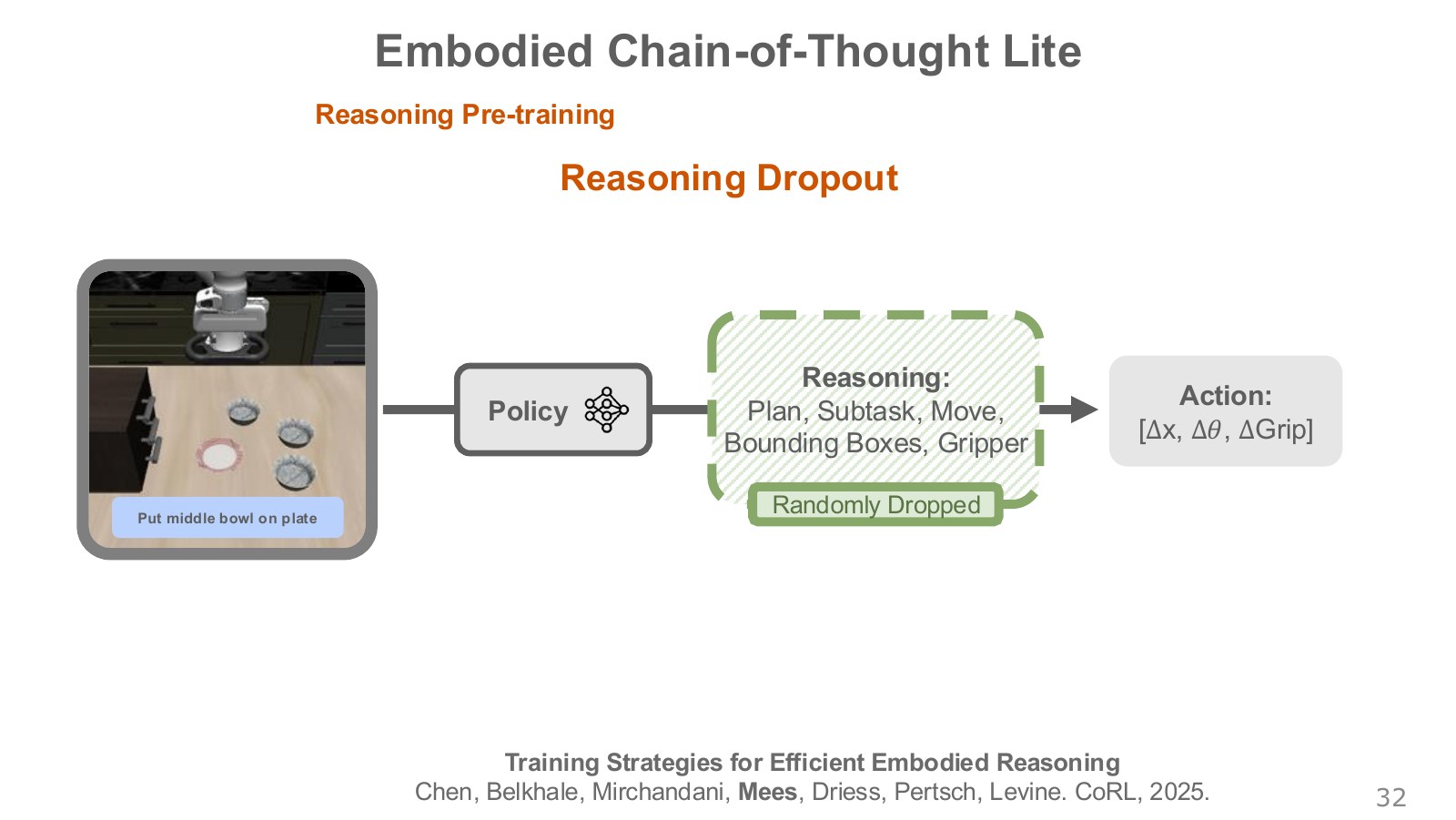
This sequence gradually reveals the same architecture. Original frames P020–P032 can be opened in order from the copy index. Reasoning pretraining on the left learns reasoning before action training; dropout on the right mixes examples with and without reasoning within one process. When reasoning is omitted, ground-truth reasoning must not secretly remain in action inputs, or training would no longer match that deployment path.

#P034 · Success and inference speed on physical WidowX

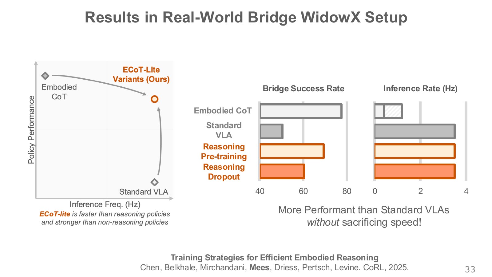
In real-robot comparisons, full ECoT has generalization-success advantages but slower policy calls, while lightweight variants trade some success for speed. Read both axes independently. More actions per second do not ensure shorter completion time, since failures and retries also take time.

#P035 · Are reasoning and action data paired?

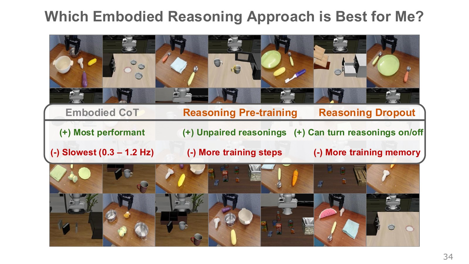
If human videos provide abundant reasoning annotations without matching robot actions, two-stage pretraining is natural. If the same robot trajectories contain both reasoning and actions, dropout can train direct-action and reasoning paths together. Deployment can choose between editable explanations and fast responses.

#Spending more computation at execution

#P036 · Beyond fixed reasoning steps: more computation for harder problems

Earlier ECoT outputs predefined kinds of intermediate information in order. Test-time scaling asks whether difficult problems can receive more candidates or reconsideration. It changes the current problem’s computation budget while holding model size and training data fixed.

#P037 · Connecting classical planning, learned planning, and language reasoning

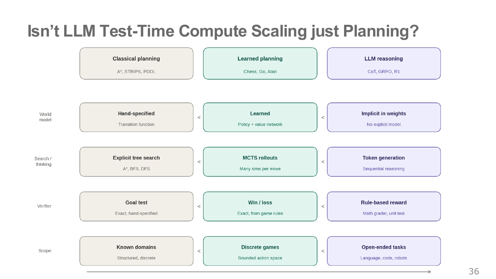
Test-time scaling generates more candidates, revises earlier answers, or compares candidates longer without updating model weights. In Go, a policy network proposes promising moves and Monte Carlo tree search (MCTS) examines continuations. The lecture’s approximately 3,000 and 5,000 Elo values come from an AlphaGo Zero comparison. This is a game with explicit rules and outcomes, and the numbers belong to its evaluation system. Original lecture, 26:35 · Slide P037 · Slide P038 · AlphaGo Zero paper

#P038 · Comparing search gains with larger Go models

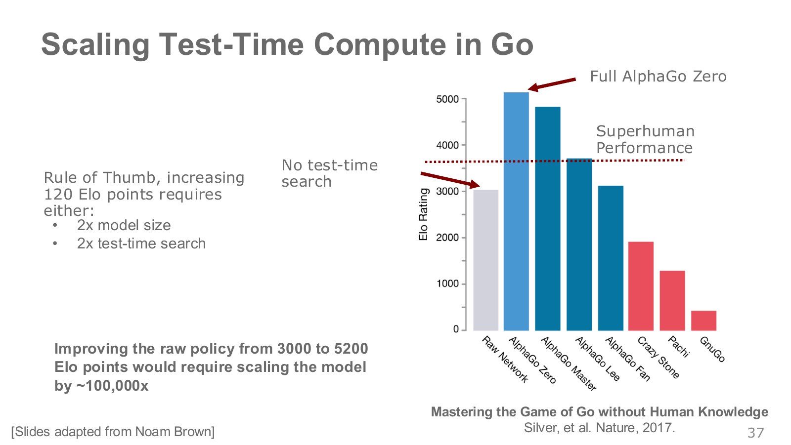
The slide’s rule of thumb associates about 120 Elo with doubling model size or search budget. Repeating it suggests roughly seventeen doublings—around a hundred-thousandfold model expansion—for a 2,000-Elo difference, conveying a dramatic cost comparison. The slide’s 3,000→5,200 and approximately 100,000× do not match this approximation exactly. Do not treat it as a validated scaling law from actually expanding the model by that amount. The point is that search delivered large gains in a well-defined game.

#P039 · Does the same trade-off hold for open-ended language problems?

Go defines legal moves and winning. “Tidy the kitchen” combines goal interpretation, object positions, and uncertain action consequences. Both useful candidate generation and correct candidate evaluation are needed.

Language models require a verifier to judge candidates. For instance, generate three drawer-opening plans and favor the one matching the observed handle position. The probability that at least one candidate is correct differs from the probability that the verifier actually selects it. The following educational calculation assumes independent candidates with identical success probabilities.

P(\text{at least one})=1-(1-p)^N

Explore the symbols and calculation The probability that at least one independent candidate is correct

Read the equation in words

For independent candidates with equal success probability, calculate the probability that all fail, then subtract it from one.

Understand each symbol

$p$: The probability that one candidate is correct.
$N$: The number of generated candidates.
$1-p$: The probability that one candidate fails.

Follow the calculation

Subtract success probability from one to obtain failure probability.
Raise failure probability to the candidate count and subtract from one.

Check with a small example

With success probability 0.2 per candidate and three independent candidates, the probability at least one is correct is $1-0.8^3=0.488$ . Verifier selection accuracy is a separate issue.

An illustrative example for understanding the equation.

#P040 · The benefit of compute budgets depends on difficulty

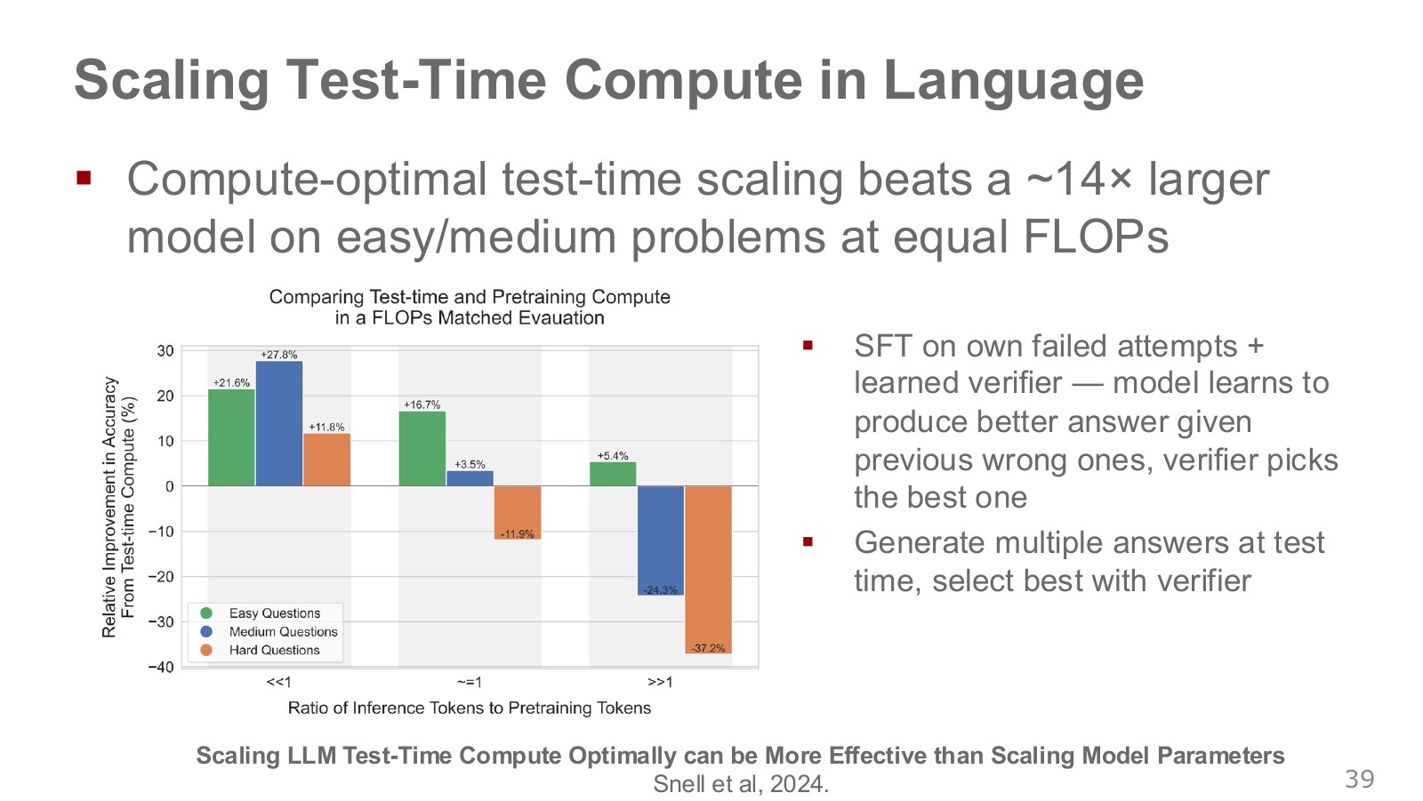
Snell and colleagues show that under equal FLOPs, smaller models allocated inference computation can outperform models about fourteen times larger on easy or intermediate problems. Hard problems can still favor larger base models. Repeated correlated wrong answers violate the independence assumption above. Robot candidate selection can also fail when a verifier mispredicts contact outcomes. Original lecture, 30:56 · Slide P040 · Snell et al.

P040’s vertical axis is relative accuracy improvement. The transcript says a decrease of up to 33.7% on hard problems, whereas this copied figure’s right orange bar reads −37.2%. It concerns the evaluated condition with a high inference-token/pretraining-token ratio, not a 37.2-percentage-point decline on every difficult problem. The intuition is that a base model must generate useful candidates for search to amplify them.

#P041 · Intermediate tokens provide space for sequential computation

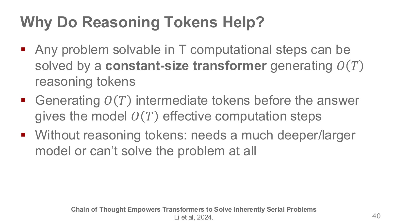
An autoregressive Transformer can output intermediate tokens and reuse them as inputs. Li and colleagues theoretically show greater sequential computation under specified assumptions. Wei and colleagues’ early CoT prompting elicits this through a few worked examples in the prompt. Model-size graphs depend on their experimental conditions and do not establish a universal size threshold for robot models. Original lecture, 33:21 · Slide P041 · Slide P044 · Li et al. · Wei et al.

P041’s theoretical claim is that a fixed-size Transformer can solve a problem requiring T sequential steps by generating O(T) intermediate tokens under specified construction assumptions. Distinguish fixed layer depth within one forward pass from computation continued by feeding tokens back. This is an existence result about a computational construction, not a guarantee that any pretrained model discovers the algorithm merely by producing longer reasoning.

#P042 · Eliciting CoT through worked examples

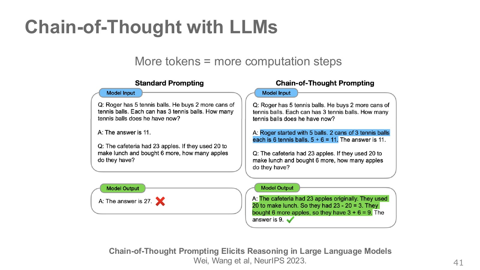
Instead of showing only “answer: 624,” original CoT prompting first gives an example explaining how to calculate weekly use and multiply by 52. The model continues similar intermediate steps for a new problem. Human examples condition the context; model weights are not updated during this execution.

#P043 · Will smaller models show the same effect?

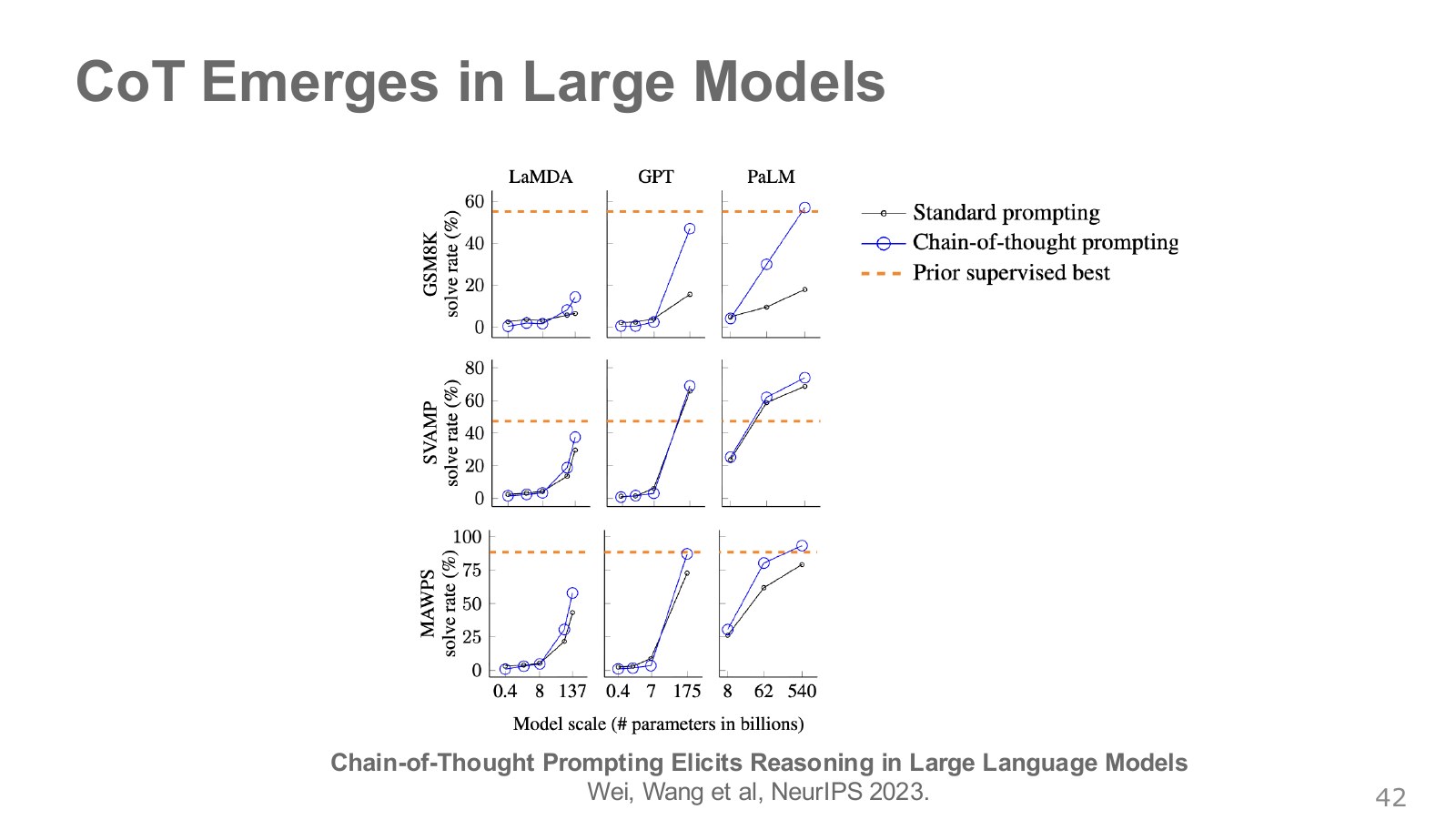
Early CoT graphs show little benefit or regressions from worked examples in smaller base models, with greater gains in larger models. The lecture’s roughly 100-billion-parameter observation belongs to those models, tasks, and prompts. Later reasoning training and distillation enable smaller models to reason too, so it is not a universal minimum size.

#P044 · Limitations of relying on human-selected examples

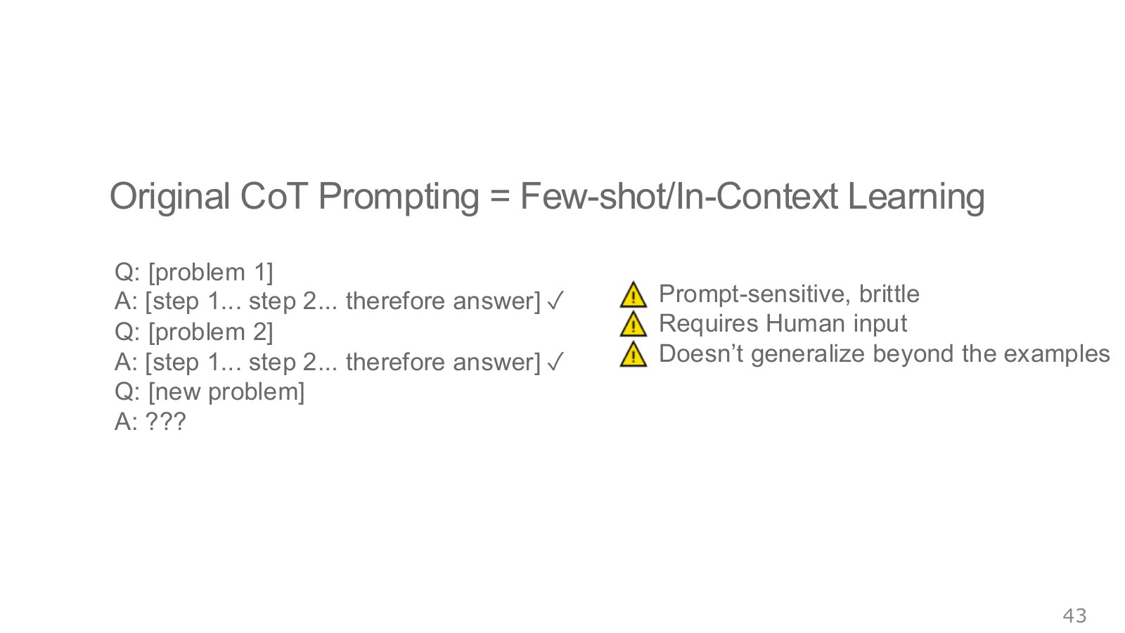
Changing example wording or order can change results, and new domains require new worked examples. This motivates another question: rather than designing reasoning prompts each time, can outcome evaluation teach the model useful reasoning strategies?

#P045 · From elicited solutions to learned reasoning strategies

#One longer attempt or several candidates?

Additional inference time can be spent differently. Revising an answer after feedback is sequential computation; generating independent answers for a verifier to select is parallel candidate search. The former uses information from previous attempts, while the latter explores several directions. Both depend on verifier scores matching the actual task.

For robots, the scene keeps changing during deliberation. If a person removes a cup or an object rolls away, a long plan based on the initial image needs updating. Recording observation time, decision completion, and execution start alongside candidate counts and accuracy helps identify where additional computation benefits the system.

#Learning reasoning through rewards for correct answers

#P046 · The letter problem: different paths to the same answer

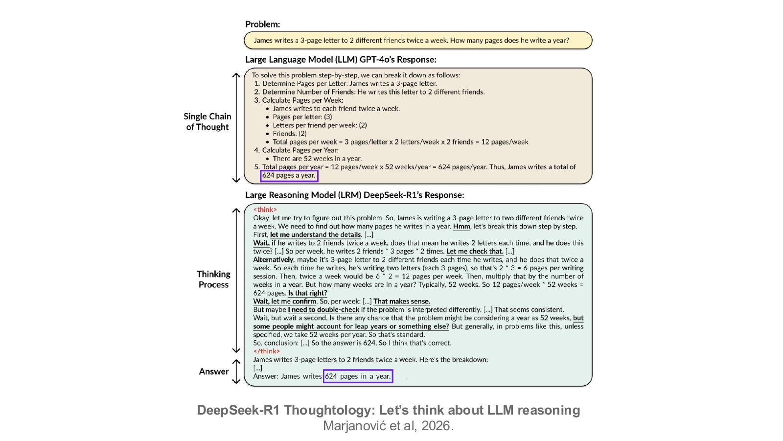
The slide asks how many pages are written in a year when sending three-page letters to two friends twice a week. Assuming 52 weeks, 3×2×2×52=624 pages. One output lists the calculation cleanly; another rechecks whether twice means per friend and verifies the interpretation and week count. Verbosity itself is not accuracy. This introduces reconsideration behavior observed in outcome-reward-trained models.

Group Relative Policy Optimization (GRPO) samples several answers to one question and compares them within the group. It updates policies similarly to PPO in Chapter 5, but uses the group’s mean score rather than a separate value estimator as its reference. The simplified example below assigns one outcome score to each response, omitting other objective terms such as PPO-style probability-ratio clipping. Original lecture, 40:18 · Slide P047 · DeepSeek-R1 paper

#P047 · GRPO: comparing answers sampled for the same question

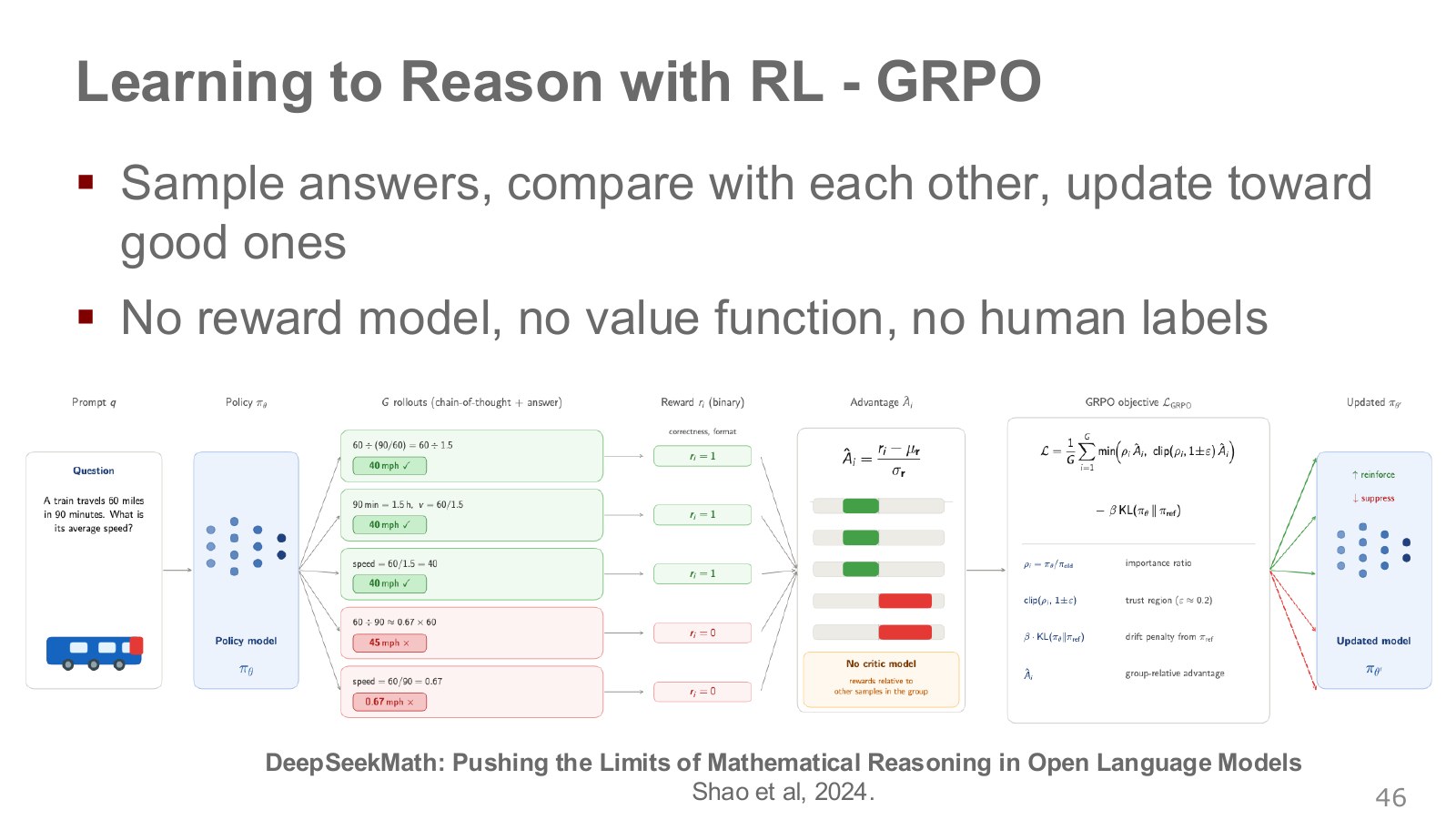
PPO used a learned critic’s expected state return as a baseline. Here, several answers to one question receive relative scores based on group reward mean and standard deviation. Four educational rewards 0,0,1,1 have mean 0.5 and population standard deviation 0.5, producing normalized scores approximately −1,−1,1,1. Updates favor better answers within the group. An answer checker must still supply reward signals.

A_i=\frac{r_i-\bar r}{\sigma_r+\varepsilon}

Explore the symbols and calculation Standardizing rewards within a group

Read the equation in words

Express how much better a candidate is than the group's mean for the same input, relative to the reward distribution's spread.

Understand each symbol

$A_i$: Candidate i's relative advantage.
$r_i$: The outcome reward assigned to candidate i.
$\bar r$: Mean reward for candidates sampled from the same input.
$\sigma_r$: The group's reward standard deviation.
$\varepsilon$: A small positive constant added in this example to avoid division by zero.

Follow the calculation

Calculate the group's reward mean and standard deviation.
Subtract the mean from each reward and divide by the stabilized standard deviation.

Check with a small example

Rewards 1,1,0,0 have mean and population standard deviation both 0.5. Ignoring the small stabilizer gives relative advantages approximately +1,+1,−1,−1.

An illustrative example for understanding the equation.

#P048 · The base model must have some chance of finding the answer

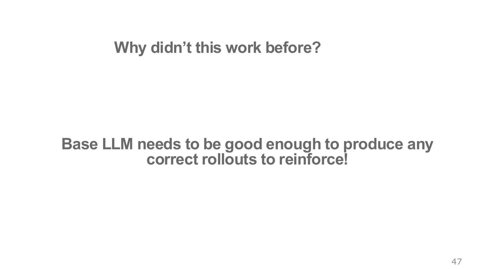
If all four answers are wrong, outcome rewards provide no relatively good answer within that group. Mees uses this to explain why a base model should occasionally solve difficult problems. Intermediate examples in R1-Zero show phrases in which the model rechecks its solution. These are observed behaviors, distinct from measured correctness across all solutions. Original lecture, 42:45 · Slide P048 · Slide P049 · DeepSeek-R1 paper

#P049 · Reconsideration behavior emerging during training

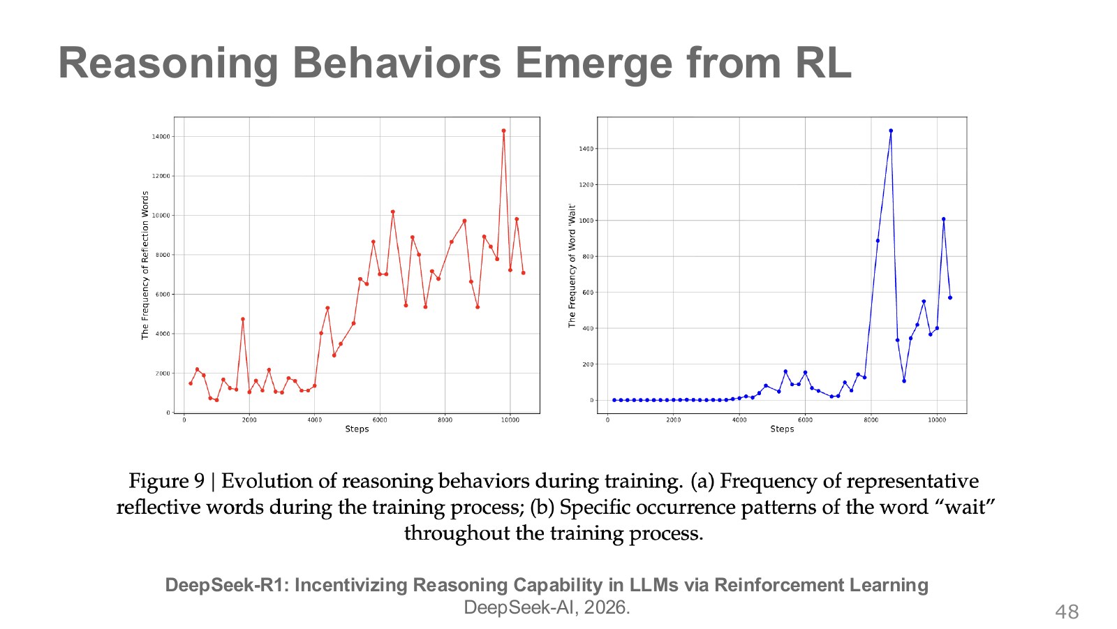
The graph shows reconsideration phrases changing in frequency with training steps. Reward optimization can reinforce these patterns without directly labeling a particular phrase. More occurrences of “wait” do not prove humanlike internal thought or causally correct reasoning. Measure solution length, correctness, and new-problem performance separately.

#What GRPO removes and what remains

Removing a value-estimation network does not remove the need to evaluate answers. Mathematics can check final-answer agreement; code can use executed tests. Verifiable rewards can reduce the expense of human grading for each solution. GRPO itself uses the provided reward signal, so the reward rule directly shapes learning.

If all four answers to a question are wrong, the group gives no preference signal. If later samples include correct answers, they receive better relative scores. The lecture’s base-capability discussion concerns this discoverable starting point. Longer outputs and more frequent correct answers are separately measurable.

#A correct answer can still misread the scene

#P050 · Can verifiable rewards extend to vision?

#P051 · Visual-RFT: box IoU instead of a mathematics checker

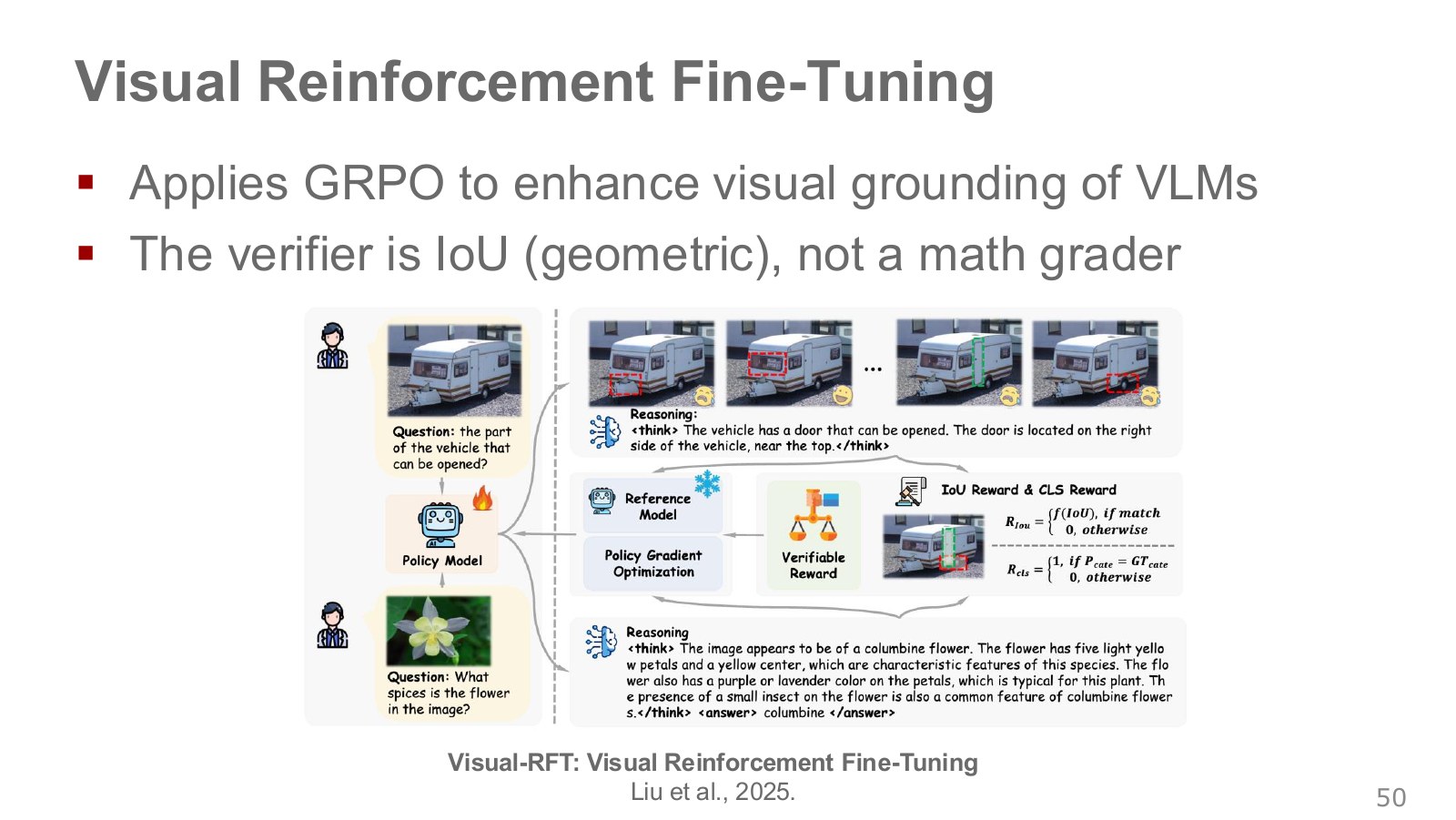
Visual-RFT scores detection boxes with intersection over union (IoU): overlapping predicted/target area divided by their union. A correct box can accompany an explanation with the wrong color or location. Box scores alone struggle to reject such explanatory errors. Original lecture, 46:31 · Slide P051 · Slide P052 · Visual-RFT paper

\operatorname{IoU}(B,\widehat B)=\frac{|B\cap\widehat B|}{|B\cup\widehat B|}

Explore the symbols and calculation Computing overlap between predicted and target boxes

Read the equation in words

Measure whether predicted and target regions identify the same location using their shared area as a fraction of their combined area.

Understand each symbol

$B$: The ground-truth region used for evaluation.
$\widehat B$: The region predicted by the model.
$\cap,\,\cup$: Intersection and union, respectively.

Follow the calculation

Calculate the boxes' intersection area.
Subtract one intersection from the sum of box areas to obtain the union, then divide intersection by union.

Check with a small example

Box areas 6 and 5 with intersection 3 give union 8, so IoU is 0.375.

An illustrative example for understanding the equation.

#P052 · A correct box and a hallucinated explanation can coexist

Imagine a model saying “the door is on the left” while correctly boxing a door on the right. IoU rewards the box without rejecting the explanation. A lucky answer or shortcut can receive the same score. A correct outcome differs from evidence genuinely grounded in the scene.

#P053 · Argos: choosing verifiers for space, time, and reasoning quality

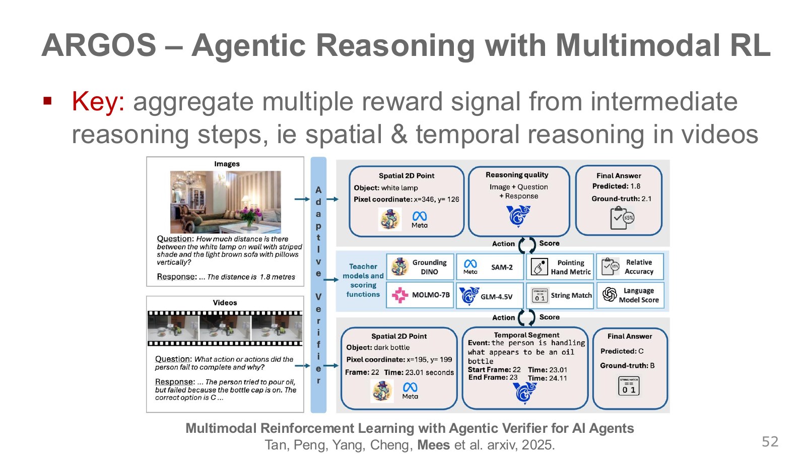
Argos selects evaluation tools per sample to construct rewards for final answers, image locations, relevant video intervals, and reasoning quality. The lecture highlights large gains under difficult ALFRED-style simulated high-level planning conditions. These evaluate decomposition and planning; immediate gripper-force adjustment during slippage requires another timescale and validation. Original lecture, 49:38 · Slide P053 · Slide P054 · Argos paper

#The cost of verifying intermediate steps

A video claim that “the person grasped the left box” must identify both its time interval and object. Argos combines localization or segmentation models, rule-based checks, and language evaluation according to the sample. This checks whether optimizing one tool’s score also passes other evaluations. Automatic verification can err too, so assess final task success alongside it. Argos team’s explanation

ALFRED-style simulated planning tests which subtask to select before moving rooms or grasping objects. Continuous arm control may need new commands at tens of hertz, making repeated long deliberation part of the performance cost. This motivates discussing ECoT-Lite alongside planning methods.

#P054 · Distinguishing better high-level plans from continuous control

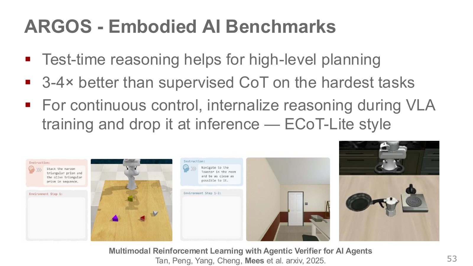
The approximately three- to fourfold improvement under difficult ALFRED conditions concerns that planning experiment against supervised CoT. It is not a multiplier for all robot-manipulation success rates. The lecture connects RL-based reasoning for slower decomposition with ECoT-Lite’s reasoning-internalized training path for fast action.

#Giving planning and control different timescales

#P055 · Four conclusions and the remaining integration problem

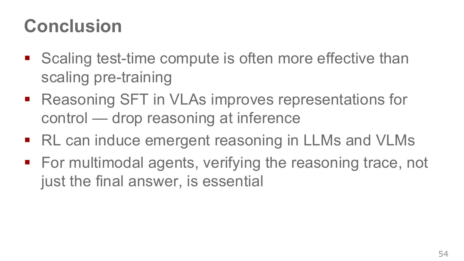
First, additional computation can be allocated at execution as well as training. Second, continuous control can learn representations through reasoning while omitting long explanations at deployment. Third, verifiable rewards can reinforce useful reasoning strategies. Fourth, multimodal models need checks of intermediate evidence alongside final answers. Integrating these into one policy that adapts and improves in the real world remains a research problem.

A high-level planner can choose a subtask such as finding a handle, opening the door, and inspecting inside, while a low-level policy rapidly adjusts hand motion as sensors update. The equation below is an educational design combining verifier scores with pre-execution waiting time. Before incorporating speed into the score, exclude candidates violating collision or workspace constraints. This two-level structure is a research direction, not experimental results from a completed ECoT-Lite–Argos system. Original lecture, 52:43 · Slide P055

J_i=v_i-\lambda d_i

Explore the symbols and calculation Including latency cost in candidate scores

Read the equation in words

An example subtracting deliberation-latency cost from verifier scores when comparing candidates that have already passed execution constraints.

Understand each symbol

$J_i$: The comparison score for candidate i.
$v_i$: The verifier score assessing compatibility with observation and task.
$d_i$: Decision latency in seconds.
$\lambda$: A coefficient assigning a score cost to one second of latency.

Follow the calculation

Read each candidate's verifier score and latency.
Multiply latency by the coefficient, subtract from the verifier score, and compare candidates.

Check with a small example

At a penalty of 0.1 points per second, score 0.9 with two-second latency becomes 0.70. Score 0.8 with 0.5-second latency becomes 0.75, so the latter is selected in this example.

An illustrative example for understanding the equation.

ETH’s same-week discussion readings include In-Context Imitation Learning, which places demonstrations in context, and Voyager, which stores code skills and revises plans in Minecraft. Reading them together distinguishes weight learning, execution-time candidate search, and reuse of execution experience. In-Context Imitation Learning · Voyager · Archit Sharma’s invited talk

The next chapter examines when unfamiliar environments call for more computation and when control should pass to a person. Chapter 11: Open Problems in Robot Learning