Let us move beyond evaluating actions and directly change the probabilities of actions that produce good outcomes. This chapter explains how to obtain policy gradients and what makes those gradients useful in practical robot learning.
Oier Mees · ETH Zurich 2026, Lecture 5 · Official lecture · Original PDF
#P001 · Policy gradients directly change the probabilities of good actions
Imagine a robot reaching toward a cup in a slightly different direction each time. What if it chose movements that happened to grasp the cup successfully more often, and movements that knocked it over less often? This chapter turns that intuition into derivatives with respect to neural-network weights.
In Chapter 04, we learned a function that scores actions and selected high-scoring actions. Here, we adjust the policy itself. A policy is a rule for choosing actions from states; a stochastic policy provides a probability or probability density for each possible action. Improving a policy means changing that distribution toward better outcomes.
Starting with the derivation of REINFORCE, we refine noisy learning signals with baselines and advantages, examine the conditions for reusing past data, and continue to PPO and SAC. Even algorithms sharing an actor–critic structure differ in how they collect data and which objective they optimize.
#P002 · The algorithm table compares information requirements and reusable data
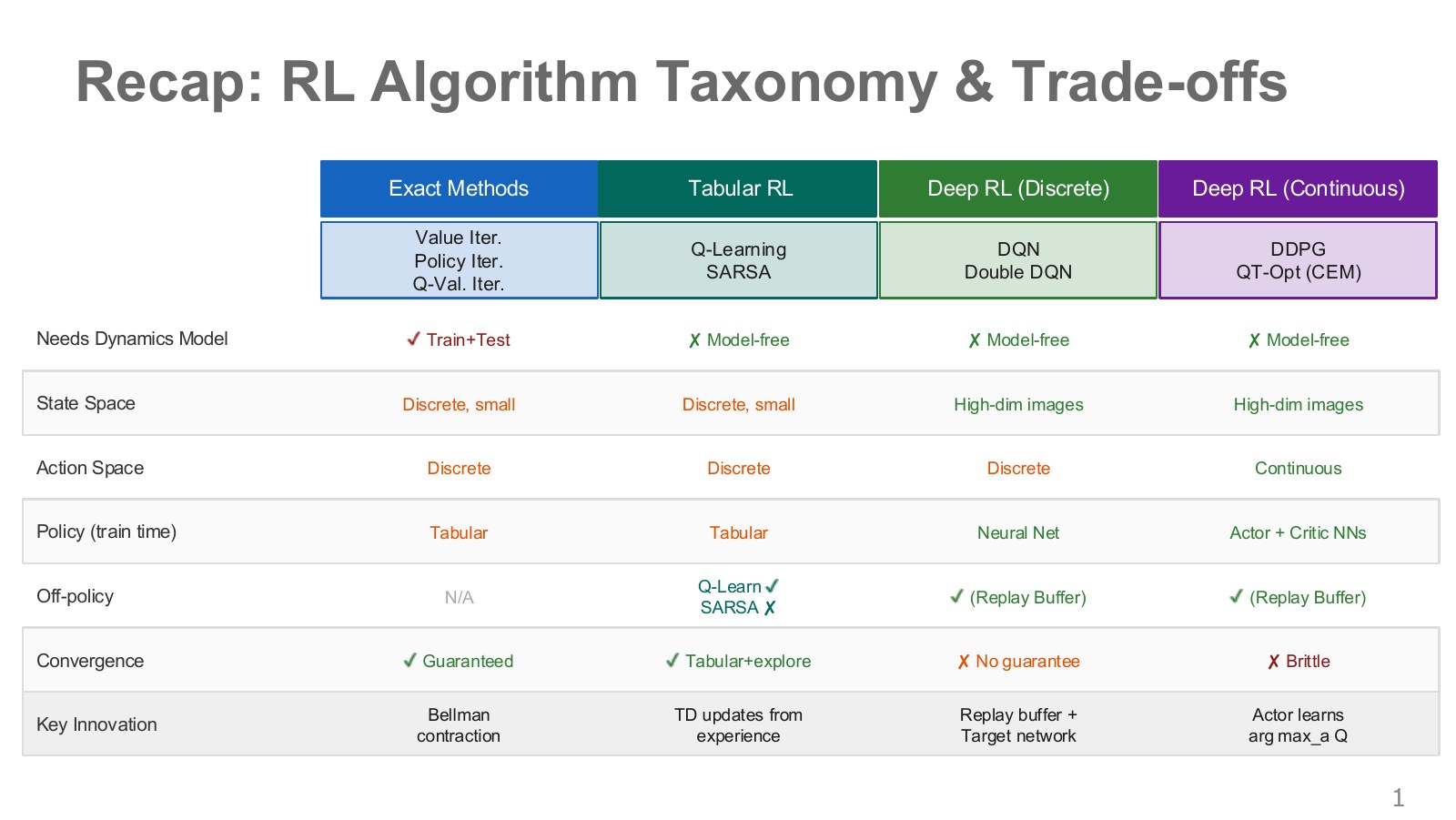
The table’s four columns cover exact computation, learning small tables, deep reinforcement learning for discrete actions, and deep reinforcement learning for continuous actions. Reading across each row reveals their information requirements. A dynamics model describes how the state changes after an action. Value iteration with a known model starts from different information than Q-learning based on stored experience.
Discrete actions are enumerable choices such as left and right; continuous actions choose real values such as joint target angles or torques. High-dimensional image inputs and continuous actions are separate properties. A policy choosing one of four directions from an image has a large input but discrete actions.
A replay buffer stores past states, actions, rewards, and next states. Q-learning methods can use past actions in updates even when those actions differ from the current policy. SARSA and basic policy gradients are more directly tied to the data distribution generated by the current policy. The table’s convergence marks rely on conditions such as a small finite MDP, sufficient visitation, and suitable learning rates. Replacing a table with a neural network does not automatically preserve those guarantees.
DDPG already has an actor, so it would be inaccurate to say that Chapter 04 contains only values and Chapter 05 introduces policy networks for the first time. We revisit the relationship here through stochastic-policy gradients and the problem of estimating them.
#P003 · Evaluate actions before choosing, or learn selection probabilities directly?
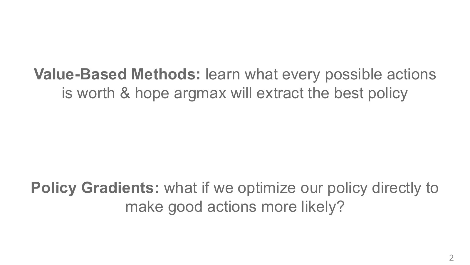
Value-based methods first ask, “How much will I receive in the future if I take this action?” Policy gradients ask, “Which policy weights should change to make actions that produced good outcomes more likely?” These approaches can compete, or they can be combined in actor–critic methods.
Weights collect the neural network’s adjustable parameters into a vector. The distribution selects action in state . A logit is a score before conversion to a probability. For example, logits of 0 and 1 for two actions become probabilities of approximately 0.269 and 0.731 under softmax: exponentiate each score and divide by their sum. For continuous actions, a network can output a mean and standard deviation defining a Gaussian distribution. A Gaussian concentrates values in a bell shape around its mean, with the standard deviation controlling its spread.
Learning a policy directly does not remove the need to evaluate future outcomes. Actual rewards or a critic still have to indicate which actions were better. Stochastic behavior alone also guarantees neither safe exploration nor sufficient experience.
#P004 · Improve expected return across repeated runs, rather than one lucky outcome
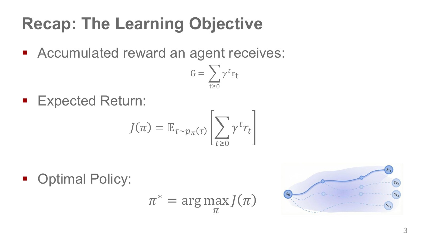
A reward is an evaluation signal at one time step; a return combines rewards across multiple time steps. If approaching a cup gives small rewards and a successful grasp gives a large reward, the return from one run adds those signals. The discount factor determines how much distant future rewards contribute.
Explore the symbols and calculation Return and expected return
Read the equation in words
Treat each trajectory's total reward as its score, then average according to the probability that the current policy generates that trajectory.
Understand each symbol
- One trajectory containing states and actions in time order. This symbol does not denote an angle.
- The reward received at one step: a learning signal defined so that larger is better.
- The length of a trajectory or sequence. Here it sets how many steps enter the sum or product.
- The parameters collecting the trainable weights of the network or policy.
- Respectively, a single trajectory's total reward and the policy's expected return.
- Add every term over the indicated range, computing one term and repeating through the end of the range.
- An expectation: an average over possible outcomes weighted by their probabilities.
Follow the calculation
- Add every reward in one trajectory to obtain its score.
- Average those scores over trajectories the current policy can generate.
Check with a small example
If two trajectories return 1 and 5 with probabilities 0.75 and 0.25, expected return is 2.
An illustrative example for understanding the equation.
Here, is a trajectory covering an entire run, is the trajectory distribution generated by the current policy, and is its average return. The branching lines on the right indicate different outcomes from the same starting point, caused by random policy choices and environment uncertainty. We must consider not just the best path but also how likely each path is.
To keep the derivation readable, the main text uses a finite horizon and an undiscounted return. Differentiating a discounted objective exactly requires consistent time-dependent discount weights. If the objective is defined as , the gradient term at the corresponding time also carries . Merely changing the reward-sum notation does not justify mixing these two objectives.
#P005 · Trajectory probability multiplies the initial state, actions, and transitions
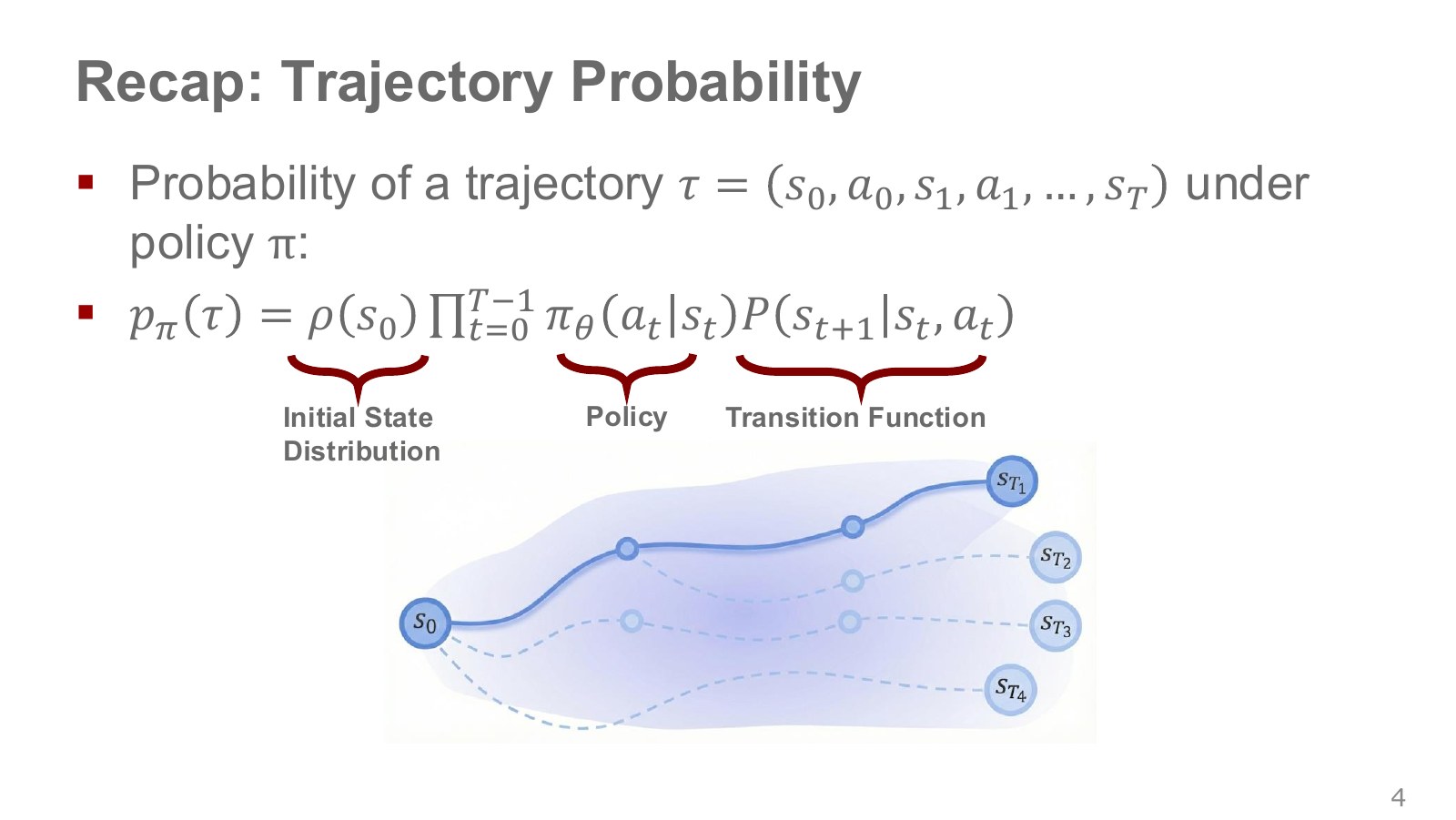
A trajectory records states and actions in time order, as in . Sample an initial state, let the policy select an action, let the environment produce the next state, and repeat.
Explore the symbols and calculation Factoring trajectory probability
Read the equation in words
Write the likelihood of the sequence of actions and states, from start to finish, as a product. Changing the policy changes action probabilities and therefore trajectory probabilities.
Understand each symbol
- One trajectory containing states and actions in time order. This symbol does not denote an angle.
- The distribution specifying an episode's initial state.
- A policy choosing actions given a state. A stochastic policy outputs probabilities or probability densities for actions.
- The probability of a next state after acting in the current state, or its density for continuous states.
- The parameters collecting the trainable weights of the network or policy.
- The length of a trajectory or sequence. Here it sets how many steps enter the sum or product.
- Multiply every term in the indicated range. This appears when computing the joint probability of successive choices.
- Conditional notation: the information to the right of the bar is given. This is not a division sign.
Follow the calculation
- Distinguish the initial-state distribution, environment-transition distribution, and policy action distribution.
- Multiply per-step action and transition probabilities together with the initial probability.
Check with a small example
For a one-step trajectory with initial, action, and transition probabilities 0.5, 0.4, and 0.8, the overall probability is 0.16.
An illustrative example for understanding the equation.
Here, is the initial-state distribution and the environment transition. The terms multiply because every step must occur to form the trajectory. Taking the logarithm turns the product into a sum, which later lets us calculate gradients for long runs.
The environment remains part of this probability even in model-free policy gradients. We assume, however, that changing policy weights does not directly change the initial distribution or environment laws. Their direct derivatives with respect to those weights therefore disappear later. This does not ignore the policy’s effect on the state distribution: that effect is already contained in the full trajectory distribution.
#P006 · Monte Carlo evaluation averages the outcomes of sampled runs
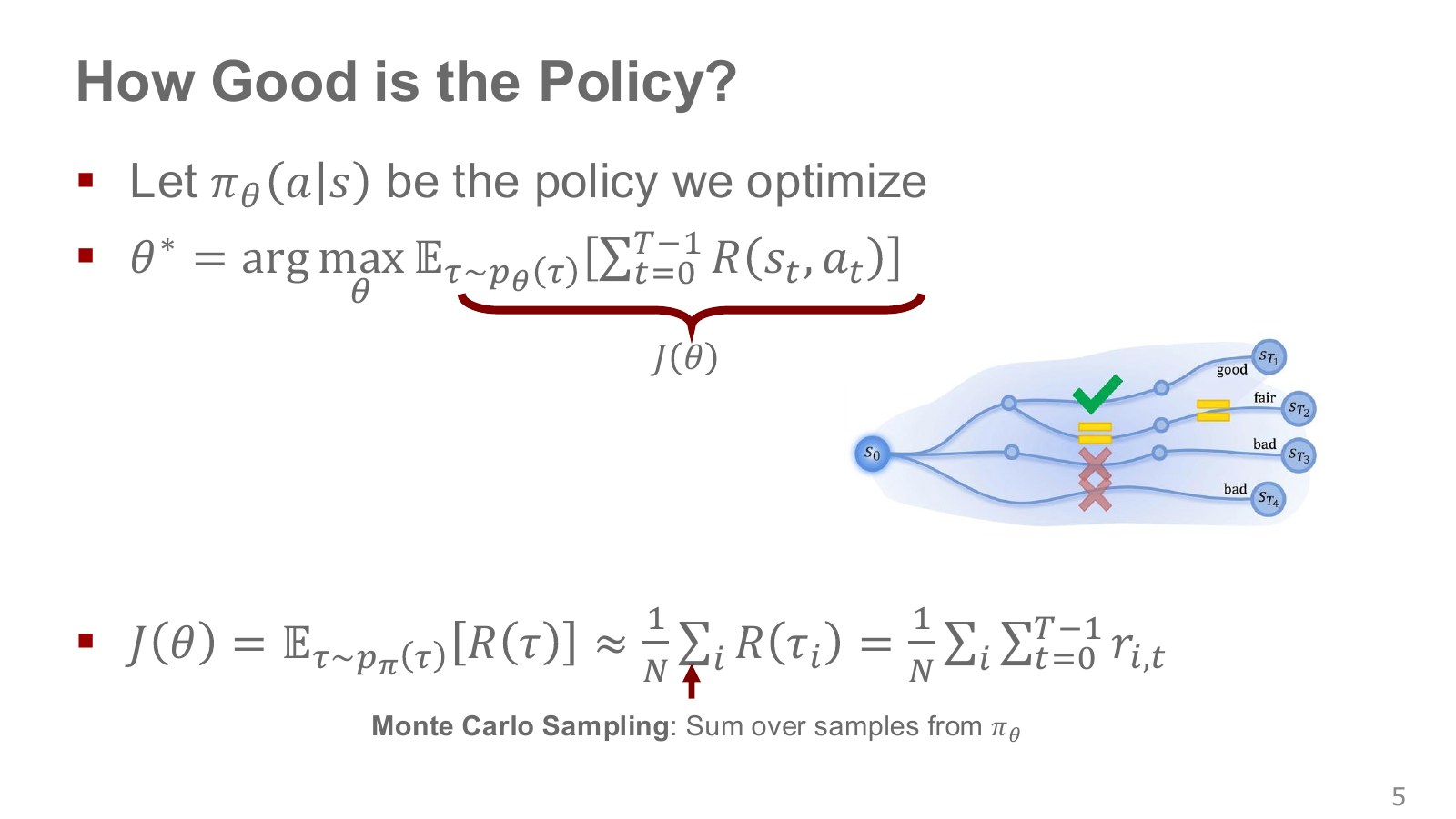
Run the robot several times under the same policy and calculate each return to estimate the policy’s average performance. Monte Carlo methods use random samples to estimate averages or integrals. We evaluate actual outcomes instead of trying to judge the policy by inspecting its network weights.
Explore the symbols and calculation Monte Carlo estimate of expected return
Read the equation in words
Since averaging every possible trajectory exactly is difficult, average the scores of trajectories actually executed. Small samples produce fluctuating estimates.
Understand each symbol
- The number of data points or samples being averaged. Dividing the sum by this count gives a per-sample average.
- One trajectory containing states and actions in time order. This symbol does not denote an angle.
- The parameters collecting the trainable weights of the network or policy.
- The estimated expected return, indicated by a hat.
- Add every term over the indicated range, computing one term and repeating through the end of the range.
Follow the calculation
- Execute the current policy multiple times.
- Add the returns from all runs and divide by the number of runs.
Check with a small example
Scores of 1, 2, and 6 across three runs give an estimated mean of 3. This sample mean need not equal the true expectation.
An illustrative example for understanding the equation.
Here, is the number of trajectories. Counting successes in ten runs and including each trajectory’s energy costs both fit this framework. More samples usually make estimates more stable, but data collected consecutively on one robot can be correlated and may not adequately represent all initial conditions.
When taking an average, the policy that collected the data matters. Simply mixing trajectories from yesterday’s different policy into an expression evaluating today’s policy creates a mismatch between the desired average and the actual sample distribution. Importance sampling, introduced later, attempts to correct that difference.
#P007 · Must differentiating rewards with respect to weights pass through the environment?
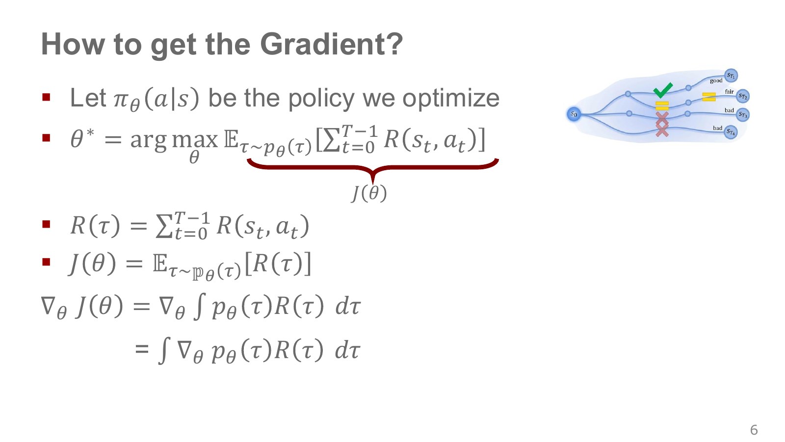
A derivative describes the direction and magnitude of an objective’s change under a small weight change. Moving weights along that gradient is gradient ascent. In ordinary supervised learning, we can backpropagate through the operations connecting the network output to the loss.
A robot moving into contact with a cup, followed by the cup slipping and the grasp failing, is not a chain consisting only of differentiable neural-network operations. Contacts may be discontinuous, and the real world’s transition rules are unknown. Yet we can still obtain a gradient for improving the policy. Instead of differentiating the numerical reward with respect to the action, we differentiate the probability of producing the action that earned it.
To do so, write expected return as an integral of trajectory probability times return. Exchanging differentiation and integration requires appropriate differentiability and integrability conditions. Linearity of integration alone does not make the exchange valid in every case.
#P008 · The log-derivative identity separates what we differentiate from what we sample
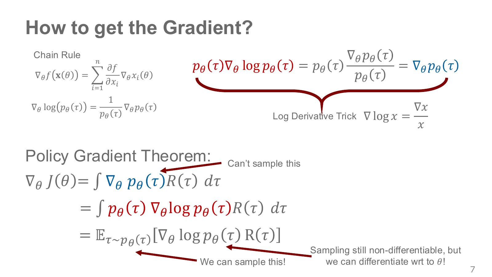
The derivative of a positive function’s logarithm equals the function’s derivative divided by the function. Multiplying both sides by the original probability density yields the following identity.
Explore the symbols and calculation The log-derivative identity
Read the equation in words
Replace a probability derivative by the probability times its log derivative. This identity enables estimating policy gradients from samples.
Understand each symbol
- The parameters collecting the trainable weights of the network or policy.
- One trajectory containing states and actions in time order. This symbol does not denote an angle.
- Trajectory probability or density depending on the weights.
- The natural logarithm. It converts products into sums and is defined only for positive inputs.
- A gradient collects componentwise derivatives describing how much the result changes when a variable changes.
Follow the calculation
- Use the fact that a log derivative equals the original derivative divided by the original value.
- Multiply both sides by the original probability and rearrange. Positive probability and differentiability are required at the point of differentiation.
Check with a small example
With probability derivative 0.1 and probability 0.5, the log-probability derivative is 0.2. Multiplying recovers the original derivative.
An illustrative example for understanding the equation.
Substituting it into the derivative of expected return gives an expectation that can be estimated with samples from the trajectory distribution.
Explore the symbols and calculation The score-function policy gradient
Read the equation in words
Multiply a trajectory's log-probability gradient by its score to make high-scoring trajectories more likely. This does not require differentiating the environment that generated the trajectory.
Understand each symbol
- The parameters collecting the trainable weights of the network or policy.
- One trajectory containing states and actions in time order. This symbol does not denote an angle.
- The direction of increasing expected return as policy weights change.
- The sum of rewards actually obtained along that trajectory.
- An expectation: an average over possible outcomes weighted by their probabilities.
- The natural logarithm. It converts products into sums and is defined only for positive inputs.
- A gradient collects componentwise derivatives describing how much the result changes when a variable changes.
Follow the calculation
- Calculate returns and log-probability gradients for trajectories collected by the policy.
- Average their products to estimate a direction that increases expected return.
Check with a small example
A sample with gradient 0.2 and return 5 contributes 1. A return of −5 instead contributes −1 in the opposite direction.
An illustrative example for understanding the equation.
Collect trajectories from , calculate for each sample, and weight it by the return. The symbol denotes the vector of partial derivatives with respect to all weights. Return is treated as a number in this calculation, so a nonsmooth reward function can still be handled when the probability distribution meets the required conditions.
This does not differentiate through the sampling operation in the ordinary way. It is a score-function estimator that differentiates how likely a sampled action is under the policy. Silver’s likelihood-ratio explanation in Lecture 7 covers the same connection.
#P009 · Action log probabilities can be computed without knowing the environment
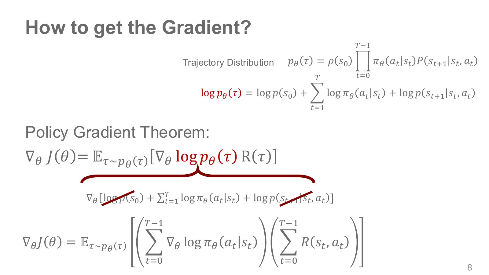
Taking the logarithm of the trajectory-probability product gives a sum of log probabilities for the initial state, each action, and each transition. If the initial distribution and environment transitions do not directly share parameters with the policy weights, their derivatives with respect to those weights are zero. What remains is the log derivative of the action probabilities produced by the policy network.
Explore the symbols and calculation Sum of action log-probability gradients
Read the equation in words
The policy-related derivative of trajectory log probability decomposes into a sum of action log-probability derivatives over time, assuming the initial distribution and environment are independent of policy weights.
Understand each symbol
- The parameters collecting the trainable weights of the network or policy.
- A policy choosing actions given a state. A stochastic policy outputs probabilities or probability densities for actions.
- The index of a step at which the robot acts in the environment, distinct from elapsed time in seconds.
- Add every term over the indicated range, computing one term and repeating through the end of the range.
- The natural logarithm. It converts products into sums and is defined only for positive inputs.
- A gradient collects componentwise derivatives describing how much the result changes when a variable changes.
- Conditional notation: the information to the right of the bar is given. This is not a division sign.
Follow the calculation
- Take the logarithm of the probability product to obtain a sum.
- Remove derivatives of initial-state and environment terms independent of the weights, leaving only action-policy terms.
Check with a small example
Log-probability gradients of 0.1 and −0.3 at two time steps give a trajectory gradient of −0.2. They are added, not multiplied.
An illustrative example for understanding the equation.
We can now proceed without an environment model. Record states, actions, and rewards on the robot, then calculate the log probabilities the policy assigns to the recorded actions. The principle is the same whether the input consists of images or joint states.
For continuous actions, is a probability density, not the probability of drawing one exact real-valued action. A density can exceed 1, and using its logarithm is normal. This estimator can nevertheless become unstable if Gaussian variance collapses to zero or log-probability calculations encounter numerical errors.
#P010 · REINFORCE repeats collection, evaluation, and policy updates
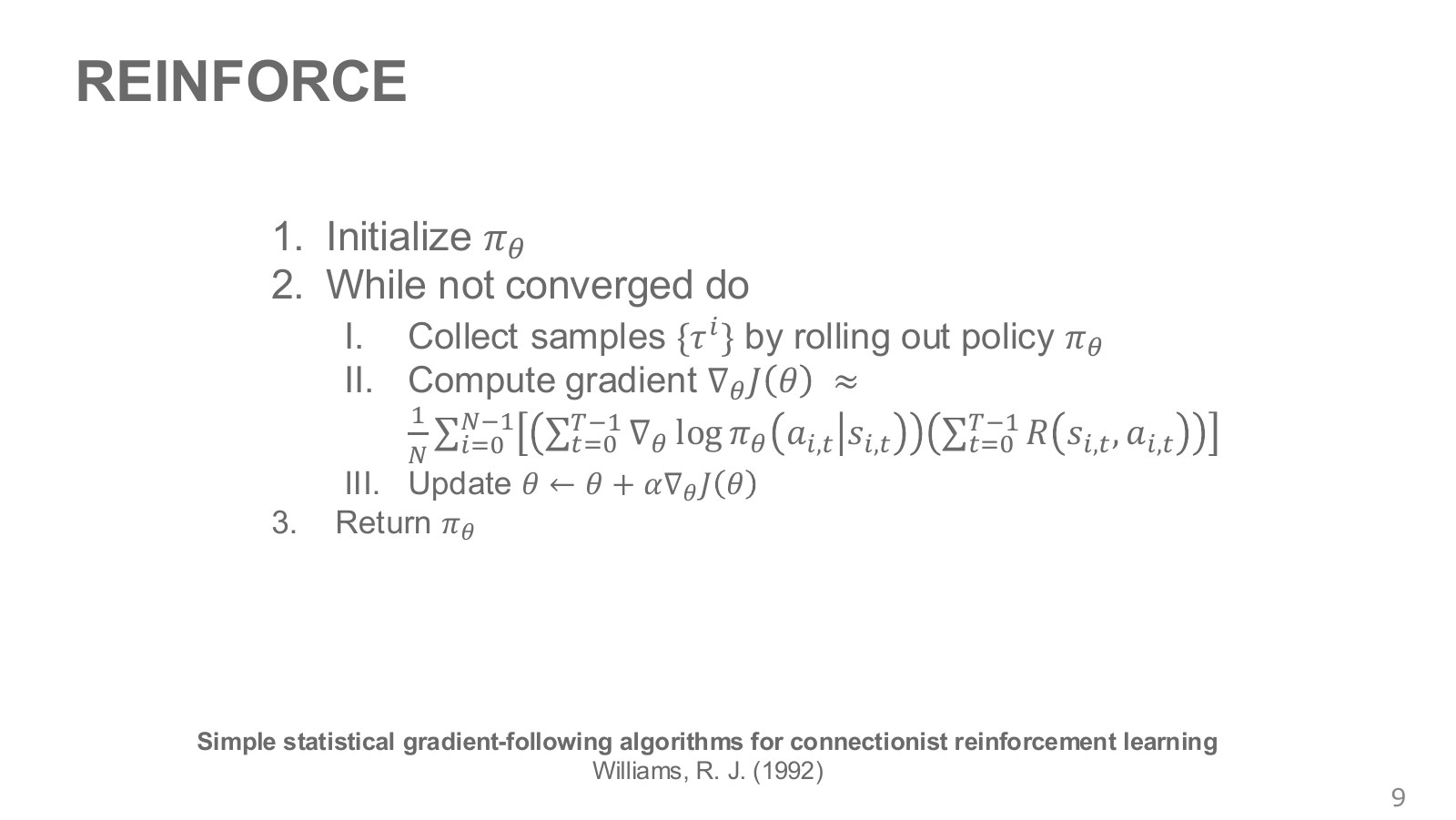
REINFORCE follows a simple sequence: collect multiple trajectories under the current policy, calculate their returns, multiply action log-probability gradients by those returns, and average. Finally, update the policy weights in that direction.
Explore the symbols and calculation REINFORCE gradient ascent
Read the equation in words
Weight each sample's action log-probability gradients by its full return, average, and move policy weights in that direction. Maximization uses an additive update.
Understand each symbol
- The parameters collecting the trainable weights of the network or policy.
- The number of data points or samples being averaged. Dividing the sum by this count gives a per-sample average.
- One trajectory containing states and actions in time order. This symbol does not denote an angle.
- The policy-gradient estimate calculated from samples.
- The learning rate controlling weight-update magnitude.
- Add every term over the indicated range, computing one term and repeating through the end of the range.
- The natural logarithm. It converts products into sums and is defined only for positive inputs.
- A gradient collects componentwise derivatives describing how much the result changes when a variable changes.
- Conditional notation: the information to the right of the bar is given. This is not a division sign.
Follow the calculation
- Within each trajectory, sum gradients across time and multiply by the return.
- Average across trajectories, multiply by the learning rate, and add to the weights.
Check with a small example
An estimated gradient of 2 with learning rate 0.01 increases the weight by 0.02. Loss-minimization code can produce the same direction by reversing the objective's sign.
An illustrative example for understanding the equation.
Here, is the learning rate. The update adds the gradient because we maximize return. With an optimizer that minimizes an objective, use a loss equal to negative log probability times return and apply gradient descent. Differentiating the return weights together with the policy can produce a different calculation from the intended score-function estimator, so those weights are usually detached from backpropagation.
Our example executes this update in a one-state, two-action problem. The good action has reward probability 0.8 and the other 0.2. We perform 1,500 updates with 64 samples each and calculate the policy’s exact expected reward at every update, separately from the observed mean return. The executable file and CSV appear later. These are not results from training robot PPO or SAC.
#P011 · Weighting a behavior-cloning-style gradient by outcomes
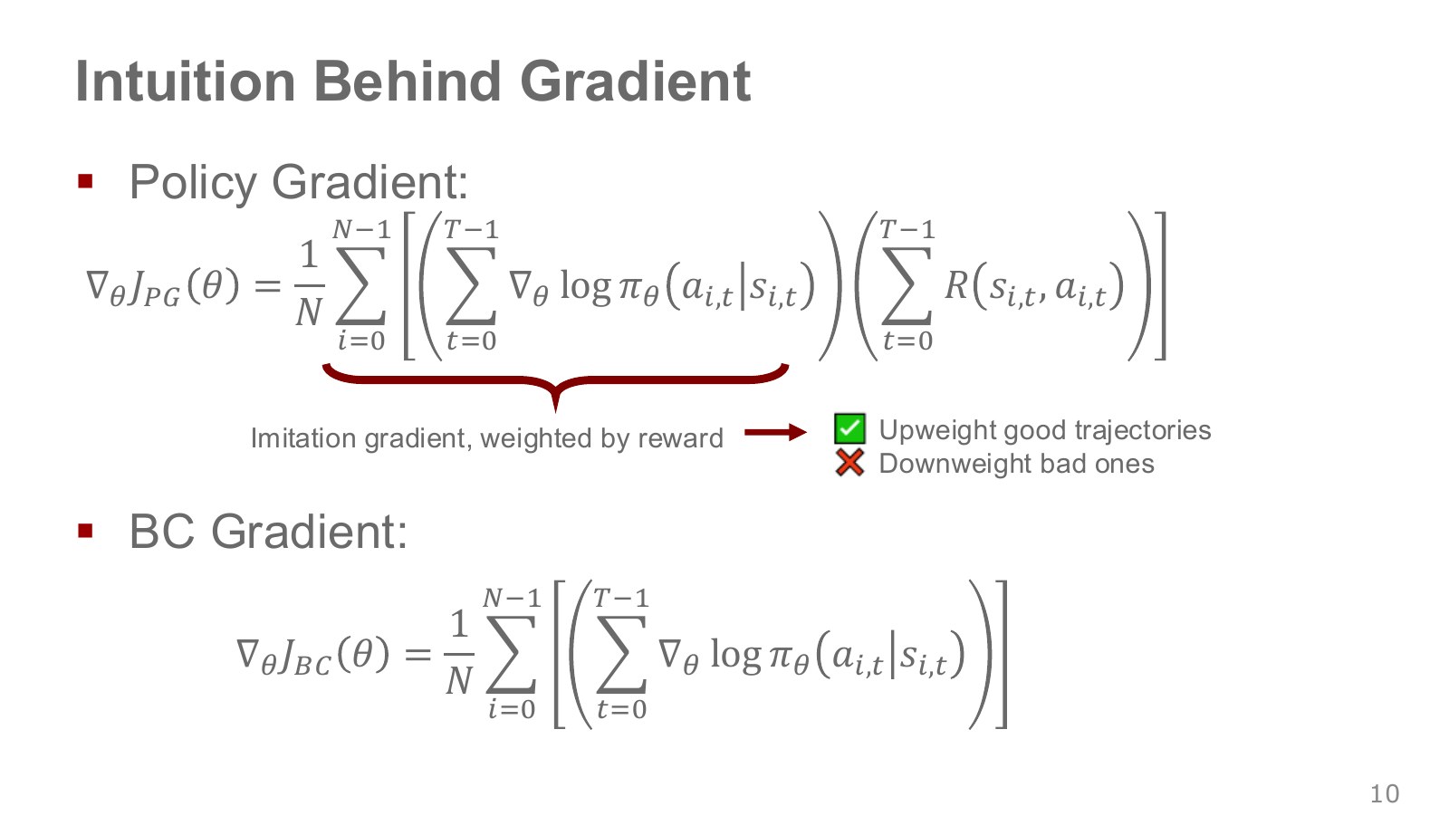
Behavior cloning learns to increase the log probability of expert actions. Its basic form does not assign each demonstration a return measuring how successful it was. REINFORCE weights actions collected under its own policy by their outcomes. To that extent, both use derivatives that make observed actions more likely.
But “increase good actions and decrease bad actions” requires a reference point. If every return is positive, trajectories returning 99 and 101 both contribute terms that increase log probability. A sample’s coefficient does not become negative simply because 99 is relatively low. Normalization among competing action probabilities and averaging across samples jointly determine the result.
Subtracting a baseline of 100, as we do later, changes the weights to −1 and +1. Only then does the intuition of reducing the probability of below-average actions directly match each sample’s sign. A similar-looking equation does not mean that inserting past expert data unchanged gives the same policy gradient.
#P012 · Future actions cannot change rewards already received
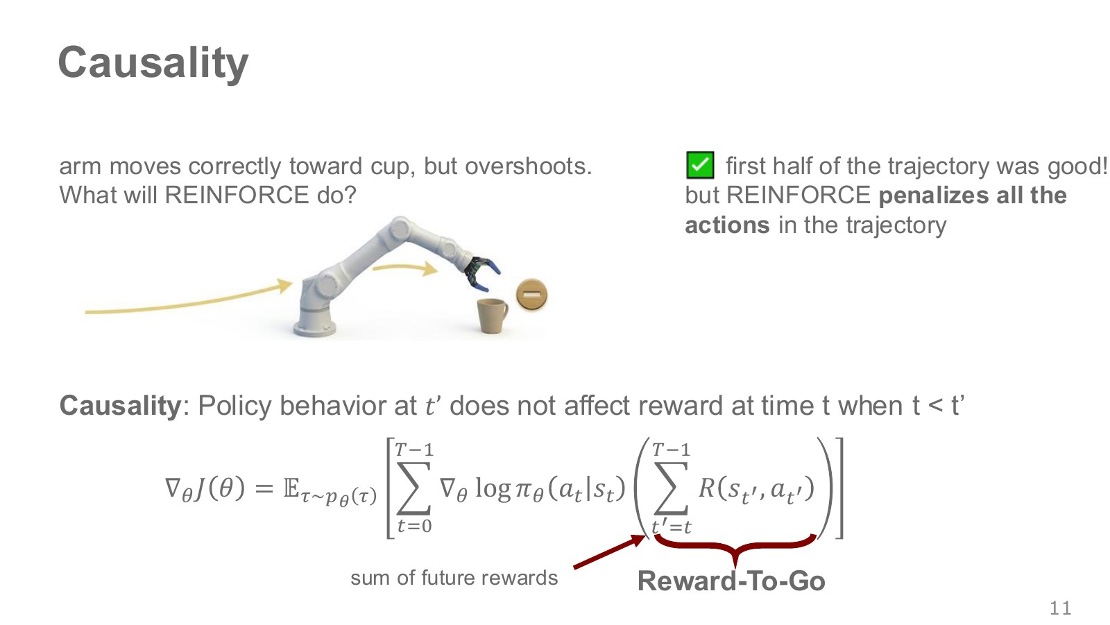
The figure shows a robot approaching a cup successfully, then moving too far at the end and losing it. Multiplying every action by the full trajectory return mixes earlier rewards unrelated to that decision into its learning signal. An action can affect only rewards from the current time onward.
In this example, weighting by the full return can also give the good early approach an unfavorable signal. Time-specific reward-to-go removes past rewards and reduces variance. Identifying which particular movement caused the failure remains a separate problem.
Explore the symbols and calculation Policy gradient with future returns
Read the equation in words
Evaluate each action using rewards from that action onward rather than past rewards. This uses the causal fact that a current action cannot change rewards already received.
Understand each symbol
- The return collecting rewards after the current time. Check the sum to see whether discounting is used and where reward counting starts.
- The reward received at one step: a learning signal defined so that larger is better.
- The parameters collecting the trainable weights of the network or policy.
- A policy choosing actions given a state. A stochastic policy outputs probabilities or probability densities for actions.
- Add every term over the indicated range, computing one term and repeating through the end of the range.
- An expectation: an average over possible outcomes weighted by their probabilities.
- The natural logarithm. It converts products into sums and is defined only for positive inputs.
- A gradient collects componentwise derivatives describing how much the result changes when a variable changes.
- Conditional notation: the information to the right of the bar is given. This is not a division sign.
Follow the calculation
- At each time step, separately sum rewards from that point to the end.
- Weight that time step's log-probability gradient by its future return.
Check with a small example
For rewards [1,2,3], the first action is weighted by 6, the second by 5, and the third by 3. This expression is undiscounted; do not insert gamma arbitrarily.
An illustrative example for understanding the equation.
Here, is the reward-to-go: rewards remaining from that time onward. Multiplying only by rewards after preserves the expected gradient because the score function has conditional mean zero given the history before the action. This removes unnecessary noise from the past.
This change does not mean that early approach movements are always judged successful. A penalty for later dropping the cup is still in an early action’s future and therefore remains in its . Reward-to-go removes past rewards; it does not perfectly assign responsibility to each action. Keeping this distinction in mind reconciles the cup illustration with the actual equation.
#P013 · Separating the difference between 99 and 101 from their large common offset
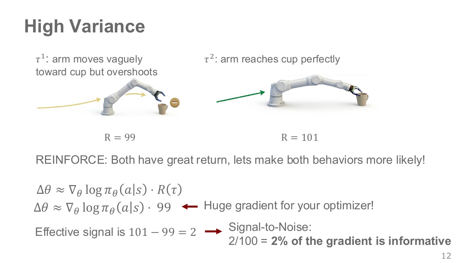
The two robot-arm illustrations compare similar high scores. Suppose one movement overshoots the cup but returns 99, while another grasps it successfully and returns 101. The difference is 2, yet each sample gradient is multiplied by a number around 100. Attaching similarly large numbers to random gradients can require many samples to estimate the mean reliably.
Here, variance measures how much gradient estimates fluctuate across repeatedly collected samples. The difference between two returns alone does not determine variance for every problem. Score-function magnitude, action probabilities, and reward noise also matter. The figure’s “2%” illustrates a contrast; it is not a general formula for measuring signal-to-noise ratio.
Subtracting a baseline removes the large common component while preserving the difference of 2. We calculate the actual variance change exactly in the small problem below. Saying that a suitable baseline helps is different from saying that every baseline always reduces variance.
#P014 · An action-independent baseline leaves the expected gradient unchanged
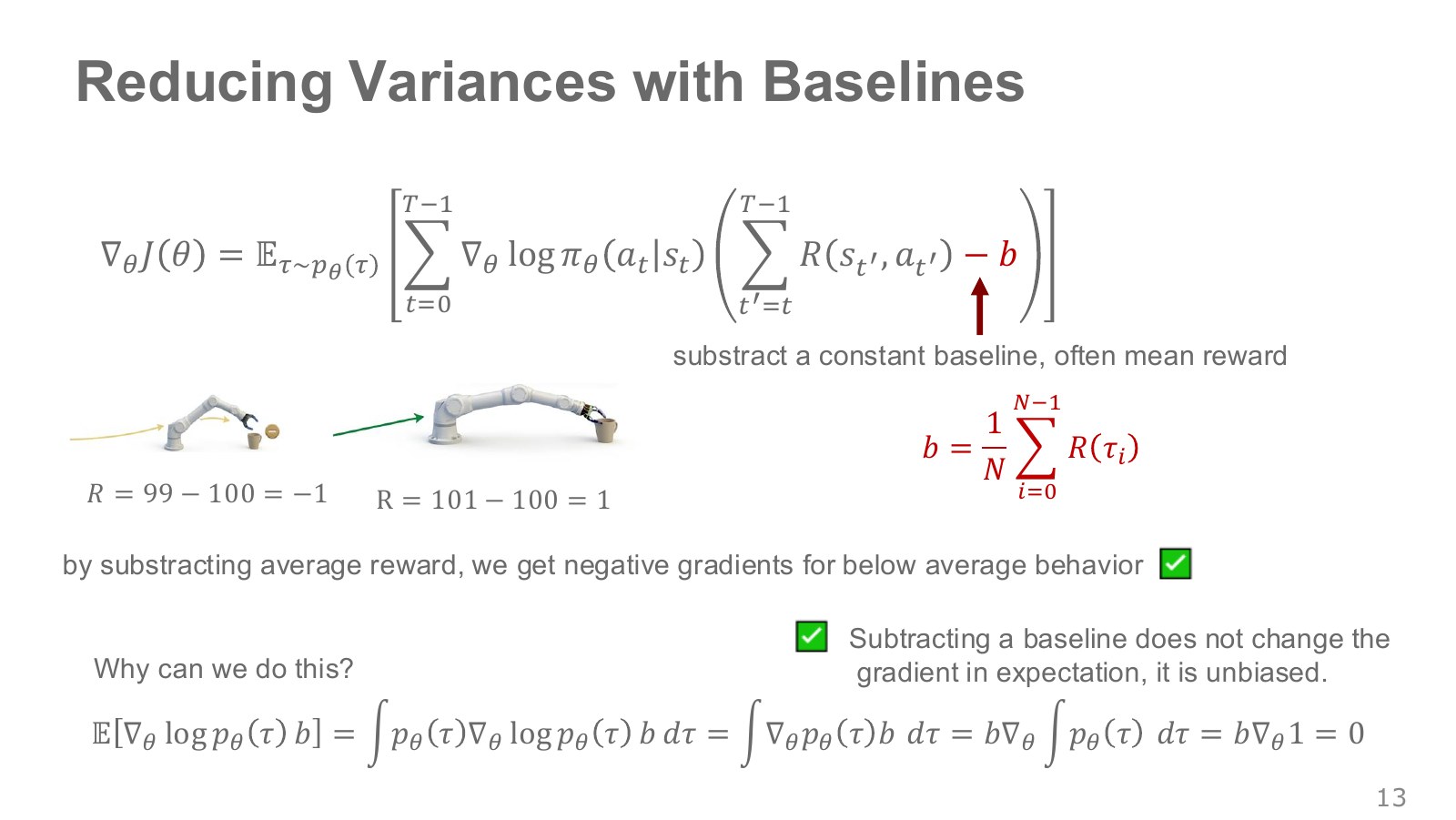
A baseline represents roughly how much return to expect in the current state. Returns above it receive positive weights; returns below it receive negative weights. Subtracting 100 from 99 and 101 gives −1 and +1, making the distinction between the actions clearer.
Explore the symbols and calculation Why the baseline term has expectation zero
Read the equation in words
Subtracting a baseline that does not depend on the current action preserves the mean policy gradient, because action probabilities sum to 1.
Understand each symbol
- A policy choosing actions given a state. A stochastic policy outputs probabilities or probability densities for actions.
- The parameters collecting the trainable weights of the network or policy.
- A baseline depending on the state but not on the currently selected action.
- Add every term over the indicated range, computing one term and repeating through the end of the range.
- An expectation: an average over possible outcomes weighted by their probabilities.
- The natural logarithm. It converts products into sums and is defined only for positive inputs.
- A gradient collects componentwise derivatives describing how much the result changes when a variable changes.
- Conditional notation: the information to the right of the bar is given. This is not a division sign.
Follow the calculation
- Move the state-only baseline outside the expectation over actions.
- Differentiating the sum of action probabilities, the constant 1, gives zero.
Check with a small example
If two action probabilities are 0.4 and 0.6 with rates of change +0.1 and −0.1, their sum's rate of change is zero. Action-dependent baselines do not permit this argument unchanged.
An illustrative example for understanding the equation.
As in Silver’s baseline explanation, this term has expectation zero, so using in the policy gradient gives the same expected gradient. The key is that the baseline does not depend on the action currently sampled. It may vary by state. Even when a baseline network is trained alongside the policy, its output is treated as a fixed weight during the actor update.
There is a subtlety when using the same minibatch’s mean return as the baseline, as illustrated in the lecture. If a sample contributes to its own baseline, the independence argument no longer applies unchanged. In a simple problem with independent trajectories, the expected estimate is scaled by . A baseline learned from separate data or a leave-one-out mean avoids this issue. Our example verifies it by exhaustive calculation for =2.
#P015 · State value provides a reference score for the current situation
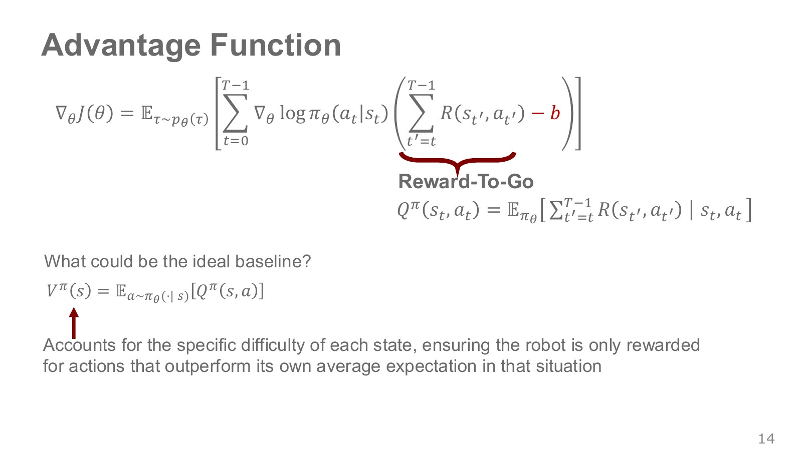
A return of 10 can be disappointing from an easy starting point and excellent from a situation that usually ends in failure. Instead of subtracting a constant 100 in every state, it is often useful to use the performance the policy normally expects in the current state.
The quantity is the expected return from taking action now and following policy afterward. The quantity is the policy’s average return from that state. Reward-to-go can be viewed as a noisy sample of this value. A state-value network learns the average from those samples and serves as a baseline.
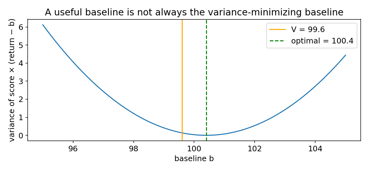
State value is not the variance-minimizing baseline for every policy. Accounting for the squared magnitude of the gradient in a single state gives the following weighted mean as the optimal constant.
Explore the symbols and calculation The variance-minimizing baseline
Read the equation in words
This shows which average minimizes fluctuations in the gradient estimate. It weights action values by squared gradient magnitude rather than taking a simple mean.
Understand each symbol
- Action value: the average return obtained by taking a particular action in the current state and then following the policy.
- The state at step , containing information such as position and velocity needed to predict what happens next.
- The log-policy gradient vector for that action.
- The state baseline minimizing gradient-estimation variance under these conditions.
- An expectation: an average over possible outcomes weighted by their probabilities.
- Conditional notation: the information to the right of the bar is given. This is not a division sign.
Follow the calculation
- Calculate the squared length of each action's log-policy gradient.
- Average action values with those weights. If the denominator is zero, the ratio cannot be evaluated directly.
Check with a small example
For action weights 1 and 3 and values 2 and 6, the baseline is .
An illustrative example for understanding the equation.
Here, . If score-function magnitudes differ between actions, this value may differ from the ordinary mean . Silver’s Lecture 7 likewise introduces as a “good baseline.” The graph below deliberately isolates this difference.
#P016 · Advantage measures improvement over the current policy's average
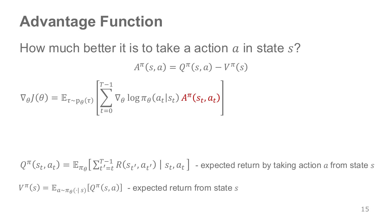
Advantage describes how much better an action is than the current policy’s average in the same state, rather than the action’s absolute score.
Explore the symbols and calculation Advantage: definition and mean
Read the equation in words
Advantage subtracts a state's average value from an action's long-term value. It measures relative benefit or disadvantage, rather than an absolute score.
Understand each symbol
- Action value: the average return obtained by taking a particular action in the current state and then following the policy.
- State value: the average return obtained by starting in a state and continuing to follow the policy.
- How much better the action is than the current policy's average action.
- An expectation: an average over possible outcomes weighted by their probabilities.
Follow the calculation
- Obtain the policy-averaged state value and individual action values.
- Subtract state value from action value; averaging under the original policy probabilities then gives zero.
Check with a small example
If action values 2 and 6 are selected equally often, state value is 4 and advantages are −2 and +2.
An illustrative example for understanding the equation.
If two actions have values 4 and 10, chosen with probabilities 75% and 25%, then is 5.5. Their advantages are −1.5 and +4.5. The simple arithmetic mean is not zero, but the mean weighted by policy probabilities is. The reference point is therefore the current policy’s average, rather than the arithmetic average over every possible action.
Subtracting a learned state value from a sampled return gives an advantage estimate. When an approximate critic replaces the exact , its error also affects the actor. Managing error and bias in exchange for lower variance becomes a central issue in actor–critic methods.
#P017 · Changing the policy also changes the data distribution
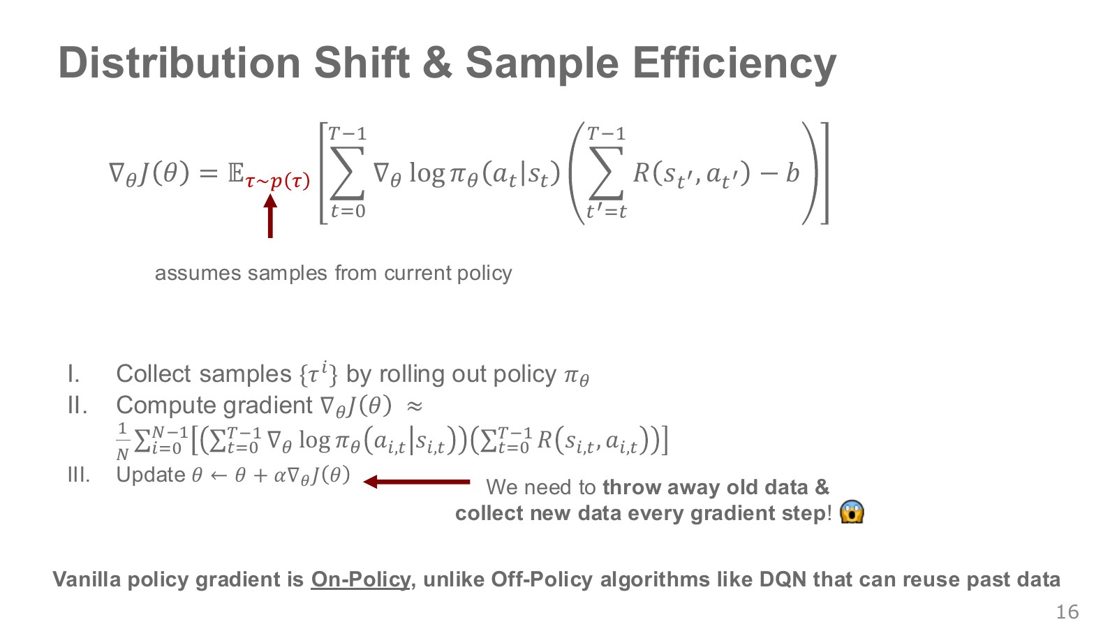
If a policy starts moving left more often, the camera sees different scenes and the robot visits different subsequent states. A dataset collected by the previous policy does not directly represent the world the new policy will encounter. This is distribution shift in policy learning.
Basic REINFORCE takes an average over trajectories of the current policy. This condition holds when calculating the gradient at the current weights on a fresh batch, but it no longer holds exactly after changing the weights and repeatedly updating on that same batch. The data need not be deleted from disk; they cannot continue to be treated as current-policy samples without correction.
Collecting real robot data takes time and entails wear and reset costs. Learning multiple times from the same data would help, but requires handling the distribution mismatch that develops during reuse. Importance sampling, small policy updates, and off-policy critics offer different approaches to this problem.
#P018 · Importance sampling corrects averages from data collected under another distribution
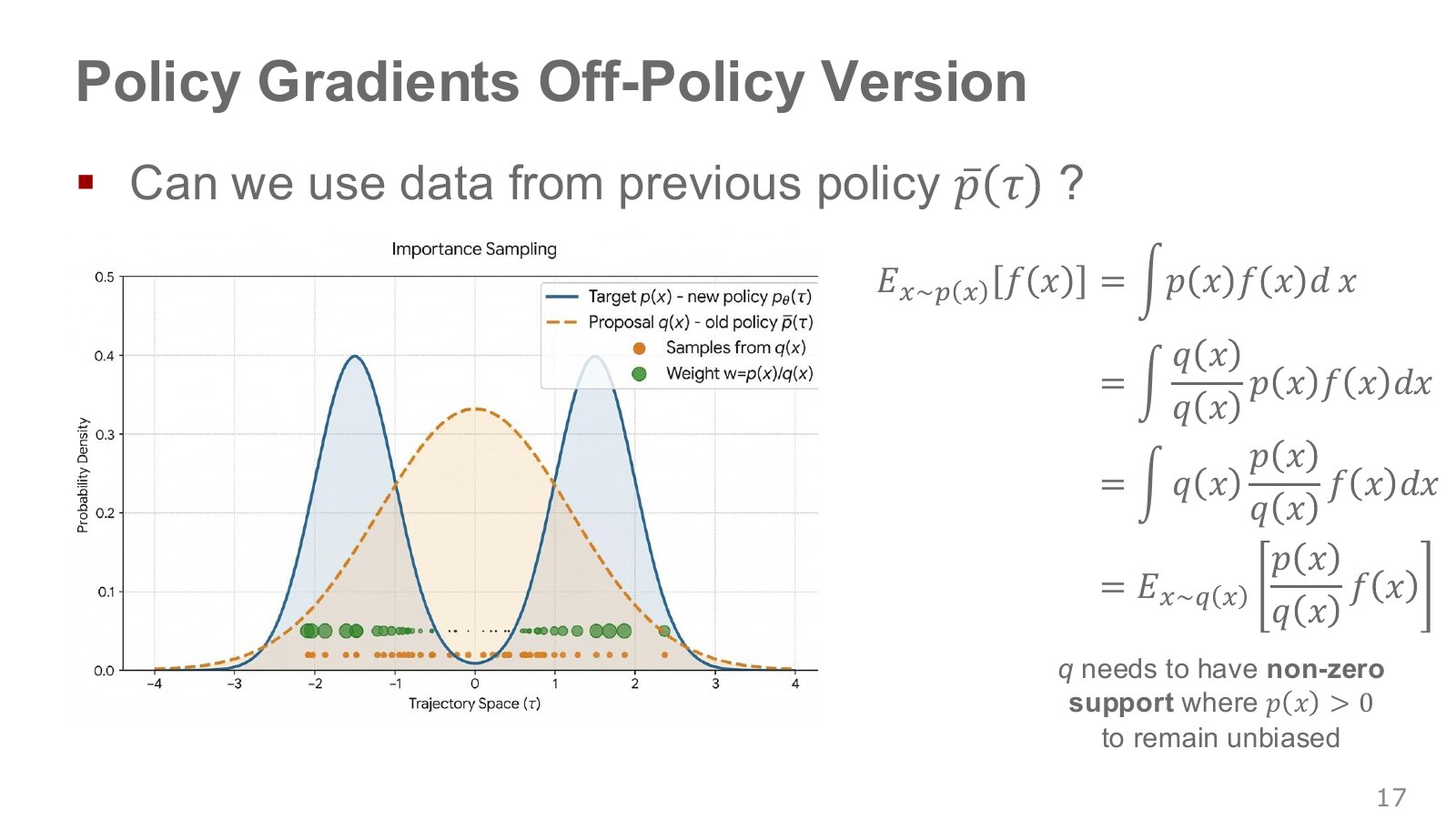
The blue distribution in the figure is the target distribution; the yellow one is the distribution actually used for sampling. Samples drawn from the yellow distribution receive larger weights when they should occur relatively more often under the target. Each weight is target density divided by collection density.
Explore the symbols and calculation The importance-sampling identity
Read the equation in words
Data from another distribution can estimate the desired mean when weighted by the new-to-old distribution ratio. The collection distribution must cover the required regions.
Understand each symbol
- Respectively, the distribution whose mean is desired and the distribution actually used to collect samples.
- The per-sample function value whose mean is desired.
- An expectation: an average over possible outcomes weighted by their probabilities.
Follow the calculation
- For each sample, divide its target-distribution probability by its collection-distribution probability.
- Multiply the function value by this ratio and average under the collection distribution.
Check with a small example
If the data distribution assigns two outcomes equal probabilities while the target assigns 0.8 and 0.2, the weights are 1.6 and 0.4. Outcomes with zero collection probability cannot be recovered this way.
An illustrative example for understanding the equation.
Suppose collection probabilities for two actions are 0.8 and 0.2, while the new policy assigns 0.4 and 0.6. If only the second action rewards 1, the collection mean is 0.2 but the target mean is 0.6. Multiplying the second action’s outcomes by 3 and the first action’s by 0.5 makes the weighted mean under the collection distribution exactly 0.6.
The identity requires a support condition: wherever the target distribution is positive, the collection distribution must also be positive. If the old policy truly assigned an action probability zero, its outcomes cannot be recovered from the data. Distinguish an outcome that happens not to appear in a finite sample from one assigned zero probability by the distribution itself.
#P019 · In the same environment, environment terms cancel in the trajectory-probability ratio
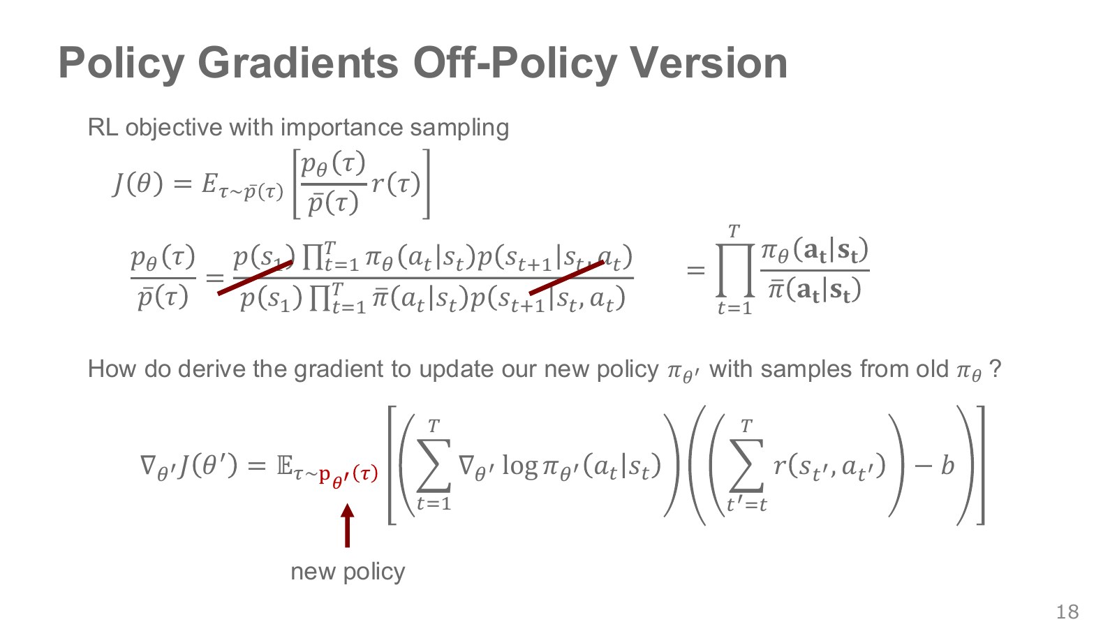
Write the previous policy as and the policy we wish to change to as . For the same trajectory collected under the same initial distribution and MDP, initial-state probabilities and environment transitions cancel between numerator and denominator.
Explore the symbols and calculation The trajectory importance ratio
Read the equation in words
Dividing a trajectory's new-policy probability by its old-policy probability yields a product of per-step action ratios. Identical initial distributions and environments cancel between numerator and denominator.
Understand each symbol
- One trajectory containing states and actions in time order. This symbol does not denote an angle.
- The previous policy used to collect the data, distinct from the new policy being updated.
- The parameters collecting the trainable weights of the network or policy.
- The importance weight for an entire trajectory.
- Multiply every term in the indicated range. This appears when computing the joint probability of successive choices.
- Conditional notation: the information to the right of the bar is given. This is not a division sign.
Follow the calculation
- Calculate new- and old-policy probabilities for every recorded state and action.
- Multiply the ratios across time to obtain the trajectory weight. Long trajectories can produce very large or small products.
Check with a small example
Two stepwise ratios of 2 and 0.5 give an overall ratio of 1. If both are 2, the product grows to 4.
An illustrative example for understanding the equation.
Saving the log probabilities that the collection policy assigned to each recorded action is enough to compute this ratio by comparison with the new policy’s log probabilities. This is why exact knowledge of the robot’s contact dynamics is unnecessary.
Berkeley Lecture 5, Part 4 also shows initial-distribution and transition terms canceling, leaving only policy-probability ratios. This cancellation assumes the same environment. If transitions differ when moving from simulation trajectories to the real robot’s distribution, policy ratios alone do not correct every difference. Data with changed reward definitions or termination conditions also cannot be treated as equivalent without explanation.
#P020 · Products of many probability ratios can give a few samples excessive weight
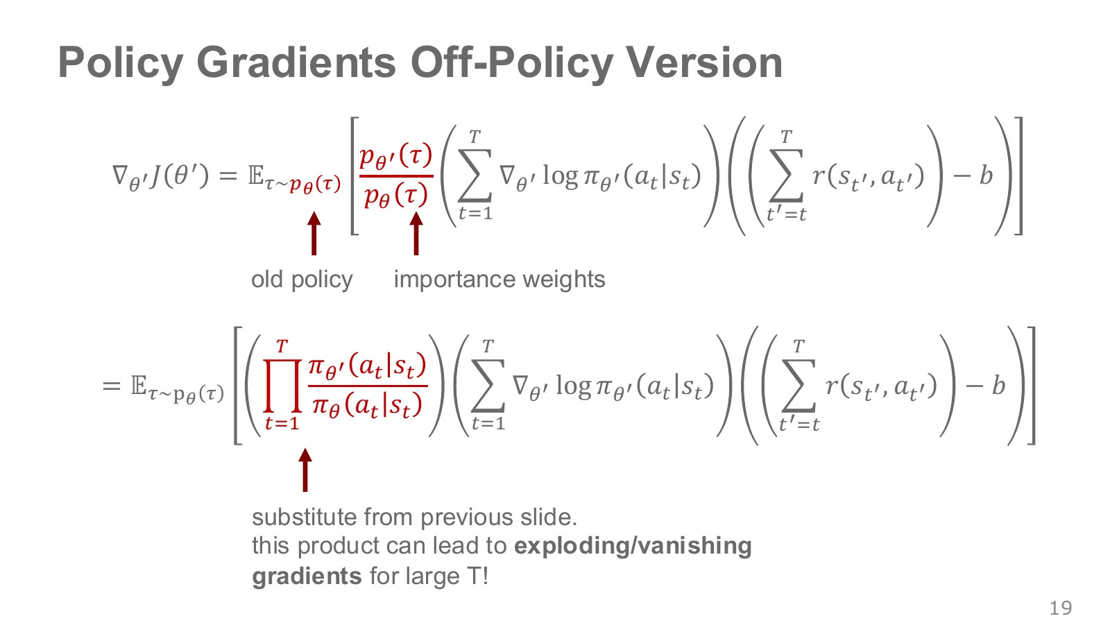
Even a per-step ratio of 1.1 becomes approximately 13,781 after 100 multiplications. A ratio of 0.9 raised to the 100th power is about 0.0000266. Small differences accumulate over long trajectories, leaving some samples almost ignored while others dominate the estimate.
This is not a theorem that all importance weights always explode exponentially. Variance depends on the policies, environment, horizon, and reward structure. Summing log probabilities can postpone numerical overflow from multiplication, but it does not solve the statistical problem of weight concentrating on a few samples.
The full trajectory weight at this stage attempts to change the distribution exactly. The later calculation retaining only a single time step’s action ratio is more convenient but introduces an additional approximation. Do not read both expressions as equally exact identities.
#P021 · Action-probability ratios alone leave changes in state visitation uncorrected
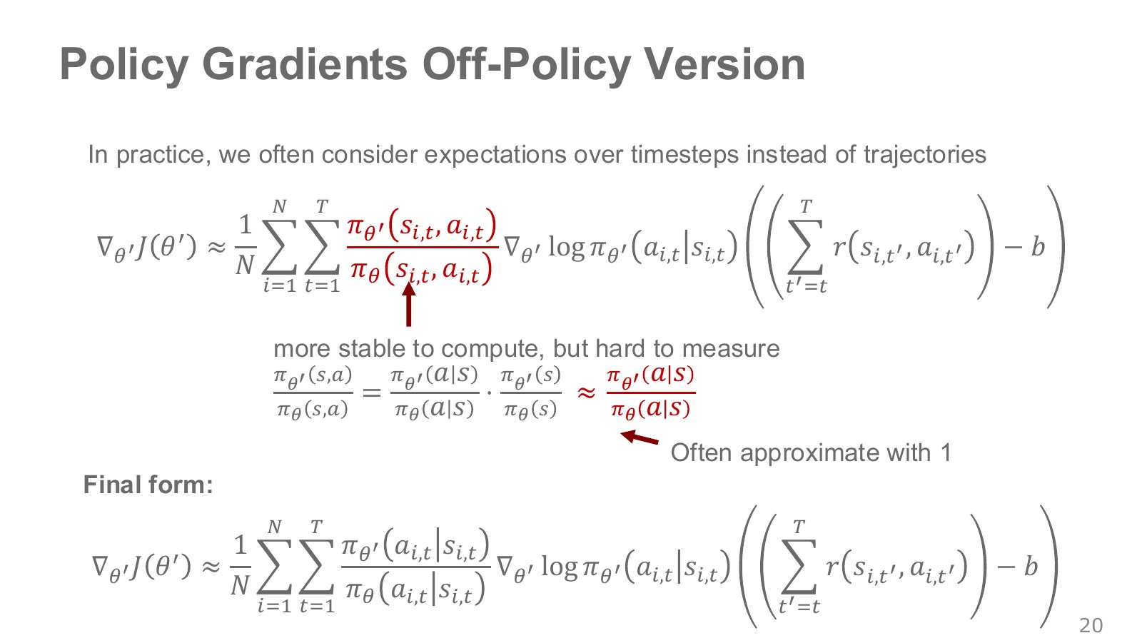
At a particular time, the probability of a state–action pair factors into the visited-state distribution and conditional action distribution. The new-to-old state–action ratio therefore also has two factors.
A single-step action ratio can be computed by feeding the same observation to both policies. But the policies may encounter that observation at different frequencies. For example, if one policy visits a corner of the workbench more often, correcting grasp probabilities in that corner does not also correct the difference in visitation frequency.
Explore the symbols and calculation State- and action-distribution ratios
Read the equation in words
Correcting action-probability ratios does not automatically correct state visitation. Changing the policy can also change which states are frequently reached.
Understand each symbol
- The previous policy used to collect the data, distinct from the new policy being updated.
- The parameters collecting the trainable weights of the network or policy.
- State-visitation distributions under the new and previous policies.
- Conditional notation: the information to the right of the bar is given. This is not a division sign.
Follow the calculation
- Separate the ratio for encountering a state from the ratio for choosing an action in that state.
- Consider both ratios to match the full state–action distribution.
Check with a small example
If a state's visitation ratio is 2 and its action ratio is 1.5, the overall ratio is 3. Using only 1.5 omits the state-distribution change.
An illustrative example for understanding the equation.
The two policy networks can compute the action-probability ratio. In contrast, describes how often a policy visits each state in the environment and cannot be obtained from one network output. Setting this ratio to 1 yields a surrogate objective evaluating the new policy’s actions at states represented by the current batch.
Fixing advantage estimates obtained under the old policy gives the practical construction leading to TRPO and PPO. It is useful near a policy that has not changed much, but an arbitrary old replay buffer does not thereby produce an exact current-policy gradient. Consider both the state-distribution approximation and differences in evaluating future returns.
#P022 · Keep the old policy fixed while reusing a batch
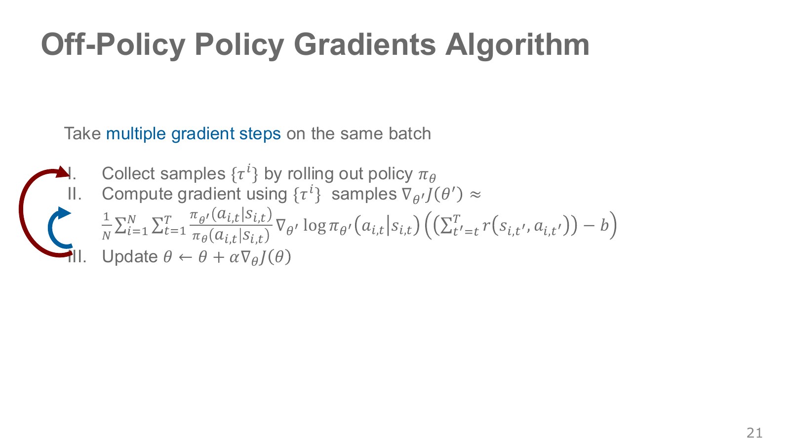
The loop-back arrow in the algorithm diagram means performing several updates on the same batch without collecting fresh data. The old policy’s recorded log probabilities must remain the same reference throughout. Replacing the denominator with the current policy at every update makes the ratio always 1, preventing it from tracking change.
Estimate returns and advantages from the collected batch, hold them fixed, and update across several minibatches and epochs. An epoch is one pass through the collected data. After enough updates, collect fresh data and reset the old-policy reference.
This differs from off-policy learning with unlimited reuse of old data. The lecture’s heading “off-policy version” marks a derivation extending the basic on-policy expression. Grouping PPO, with its approximations and restrictions, together with algorithms such as DQN and SAC that keep learning from a replay buffer obscures their different data-use strategies.
#P023 · Entropy controls how strongly the action distribution concentrates on one choice
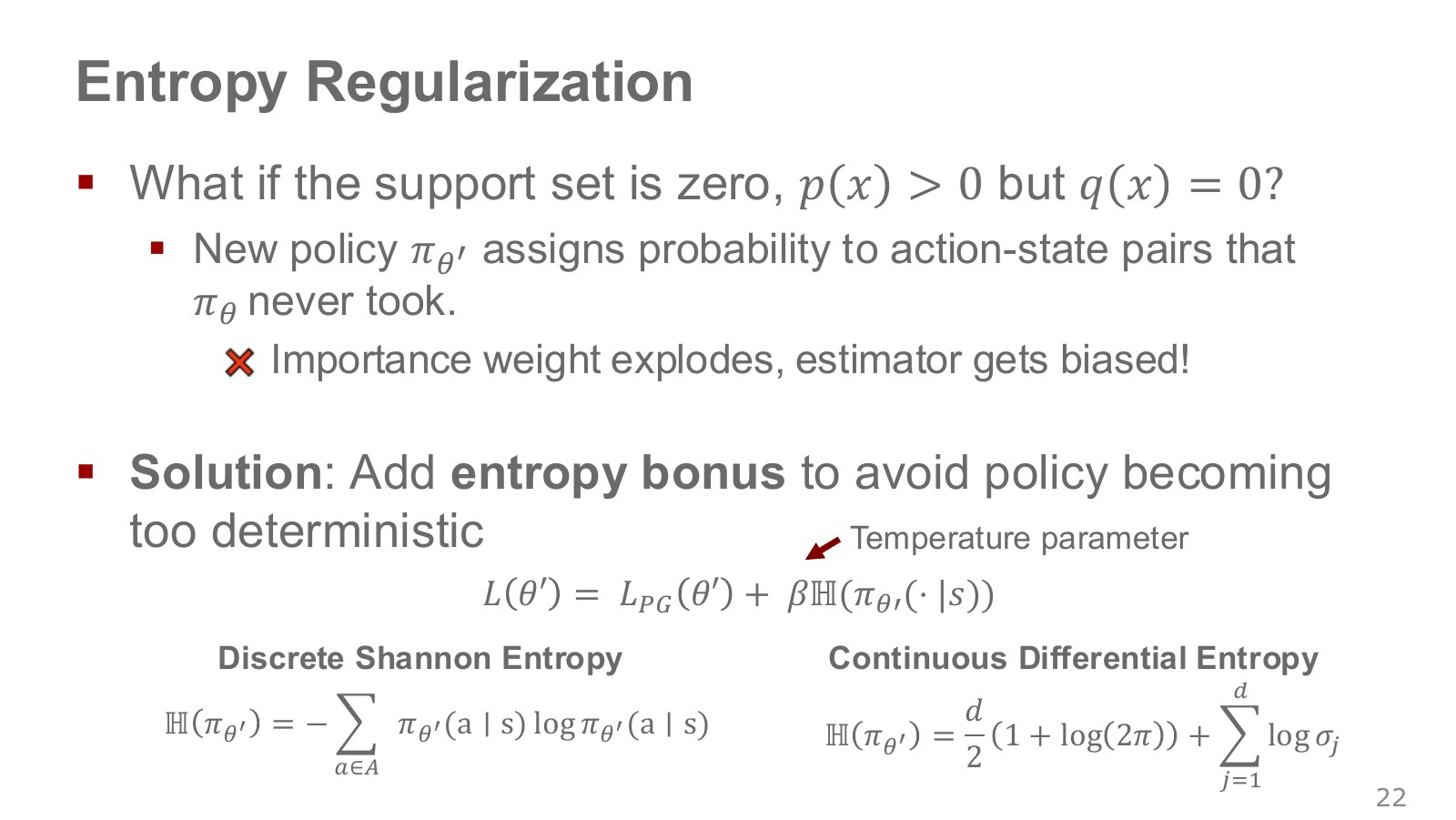
Entropy quantifies how spread out a distribution is. Choosing each of two discrete actions with probability 50% gives entropy approximately 0.693 in natural-log units; effectively choosing only one gives entropy near zero. An entropy bonus can help sustain exploration when reward maximization would otherwise concentrate the policy too early.
Explore the symbols and calculation Discrete entropy
Read the equation in words
Measure how evenly the policy distributes probability across its actions. For a discrete distribution, one certain choice gives zero entropy; more even choices give greater entropy.
Understand each symbol
- A policy choosing actions given a state. A stochastic policy outputs probabilities or probability densities for actions.
- The policy's discrete entropy at a fixed state.
- Add every term over the indicated range, computing one term and repeating through the end of the range.
- The natural logarithm. It converts products into sums and is defined only for positive inputs.
- Conditional notation: the information to the right of the bar is given. This is not a division sign.
Follow the calculation
- Multiply each action probability by its natural logarithm.
- Sum the terms and reverse the sign. A zero-probability term is defined as zero by its limit.
Check with a small example
Choosing two actions equally gives entropy approximately 0.693 nat. Assigning one action probability 1 gives zero. Entropy of a continuous density has different properties.
An illustrative example for understanding the equation.
For a diagonal Gaussian over continuous actions, differential entropy is proportional to the sum of log standard deviations. Differential entropy can be negative and depends on units and coordinate transformations, so its numerical value should not be directly compared with discrete entropy.
Adding entropy does not ensure that every unvisited state will be reached or automatically solve importance sampling’s support problem. Spreading actions within a state and reaching that state in the environment are separate issues. Since dangerous actions can also become more likely, physical robots require additional design such as command limits and stopping conditions.
#P024 · Measure policy change in action distributions rather than weight distance
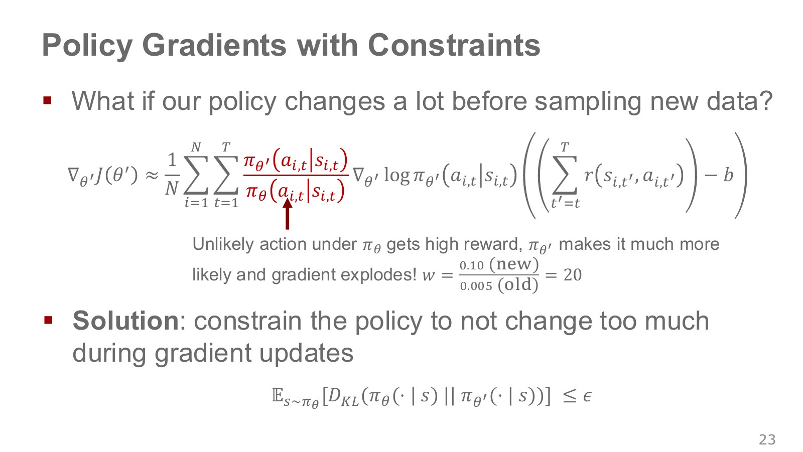
In the figure, an action assigned probability 0.005 by the old policy receives 0.10 under the new policy, giving a ratio of 20. This illustrates how one rare high-scoring experience can be amplified excessively over repeated updates. Small changes in network weights do not guarantee small changes in the action distribution.
KL divergence measures how much two distributions differ. The KL from the old policy to the new policy becomes large when the new policy makes previously possible actions almost impossible.
Explore the symbols and calculation KL divergence from the old policy to the new policy
Read the equation in words
Measure how the new policy differs from the old by averaging under the old policy's action probabilities. This is not a simple sum of probability differences.
Understand each symbol
- The previous policy used to collect the data, distinct from the new policy being updated.
- The parameters collecting the trainable weights of the network or policy.
- KL divergence comparing two distributions. It is nonnegative and generally changes when the direction is reversed.
- Add every term over the indicated range, computing one term and repeating through the end of the range.
- The natural logarithm. It converts products into sums and is defined only for positive inputs.
- Conditional notation: the information to the right of the bar is given. This is not a division sign.
Follow the calculation
- Take the logarithm of old probability divided by new probability.
- Weight by the old action probabilities and sum. A new probability of zero can make the divergence infinite.
Check with a small example
Changing [0.5,0.5] to [0.75,0.25] gives KL approximately 0.144 nat. Identical distributions give zero.
An illustrative example for understanding the equation.
KL generally changes when its direction is reversed, so it is not an ordinary distance. A small average KL across states also does not mean that every action ratio in every state lies within a fixed range. It is more accurately understood as a statistical constraint on average policy change.
#P025 · TRPO seeks expected improvement while restricting policy change
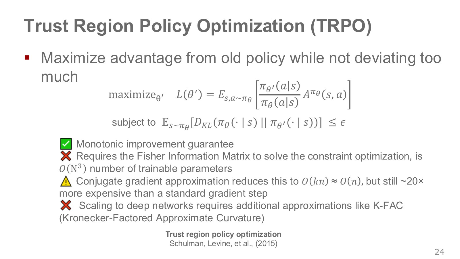
TRPO increases the product of the new-policy probability ratio and old-policy advantage at states and actions collected by the old policy. At the same time, it constrains average KL under the old state distribution to remain below a threshold. That threshold determines the size of the trust region.
Explore the symbols and calculation The TRPO surrogate objective
Read the equation in words
Construct a surrogate objective encouraging higher probabilities for actions that were advantageous in the previous data. TRPO separately imposes a KL constraint on policy change.
Understand each symbol
- New-policy action probability divided by old-policy probability. In this equation, it is not a motor input.
- An estimated advantage indicating how much better this action is than the state's average.
- The parameters collecting the trainable weights of the network or policy.
- The previous policy used to collect the data, distinct from the new policy being updated.
- An expectation: an average over possible outcomes weighted by their probabilities.
- Conditional notation: the information to the right of the bar is given. This is not a division sign.
Follow the calculation
- Calculate the new-to-old probability ratio for a recorded action.
- Multiply the ratio by estimated advantage and increase the average. The KL constraint is omitted from this line alone.
Check with a small example
For advantage 2, raising the ratio from 1 to 1.1 raises this sample's score from 2 to 2.2. Allowing arbitrarily large ratio changes is not the full TRPO setup.
An illustrative example for understanding the equation.
The original TRPO paper derives improvement guarantees from a lower bound on policy performance, then uses average KL, sample estimates, and local approximations in its practical algorithm. The slide’s “monotonic improvement guarantee” should therefore not be read as a promise that return increases in every actual neural-network run.
Berkeley Lecture 9, Part 4 adds context on natural gradients and matrix–vector computations. Explicitly constructing and inverting the Fisher information matrix, which describes curvature, is expensive with many parameters. The original paper’s practical implementation approximates a direction using matrix–vector products and conjugate gradients without explicitly constructing the matrix, then adjusts the step through line search. The lecture’s “about 20×” depends on the implementation and problem; it is not a fixed computational law. K-FAC is not a mandatory extra step in every TRPO implementation either.
#P026 · Rough-terrain locomotion depends on both joint sensing and the training environment
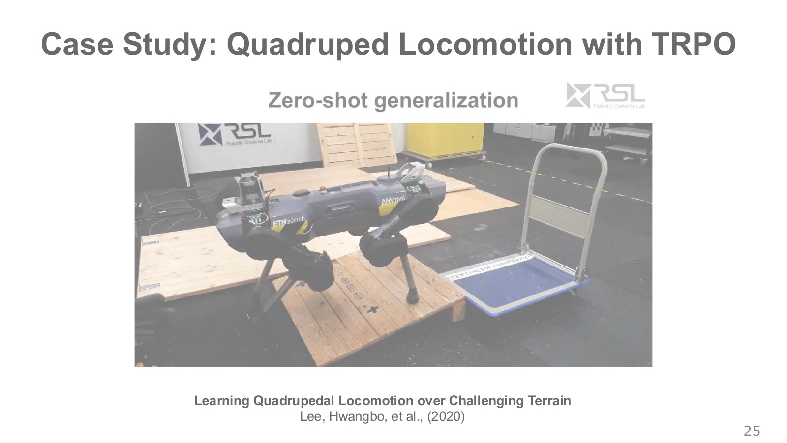
The photograph shows a quadruped negotiating ledges and obstacles. Having four legs does not automatically confer terrain understanding. Maintaining balance requires quickly using information such as whether a foot slips after contact, whether the body tilts, and whether joints track their target angles.
The 2020 work by Lee, Hwangbo, and colleagues first trained a teacher policy through reinforcement learning in simulation, with access to additional terrain and contact information. They then distilled it into a student policy receiving only histories of proprioceptive signals from joint encoders and an IMU available on the real robot. An IMU is an inertial sensor measuring signals related to body rotation and acceleration. The student learns to imitate the teacher’s actions and internal representations.
Zero-shot means deployment without retuning the policy for each test terrain. It does not mean that training data or simulation design were unnecessary. The paper combines a terrain curriculum, a physics model, and sensory-history processing. Reducing this result to “insert the TRPO equation and walk on any terrain” removes essential conditions. Read it within the actual evaluation scope of the original paper.
#P027 · PPO cuts off further gains when a favorable change becomes too large
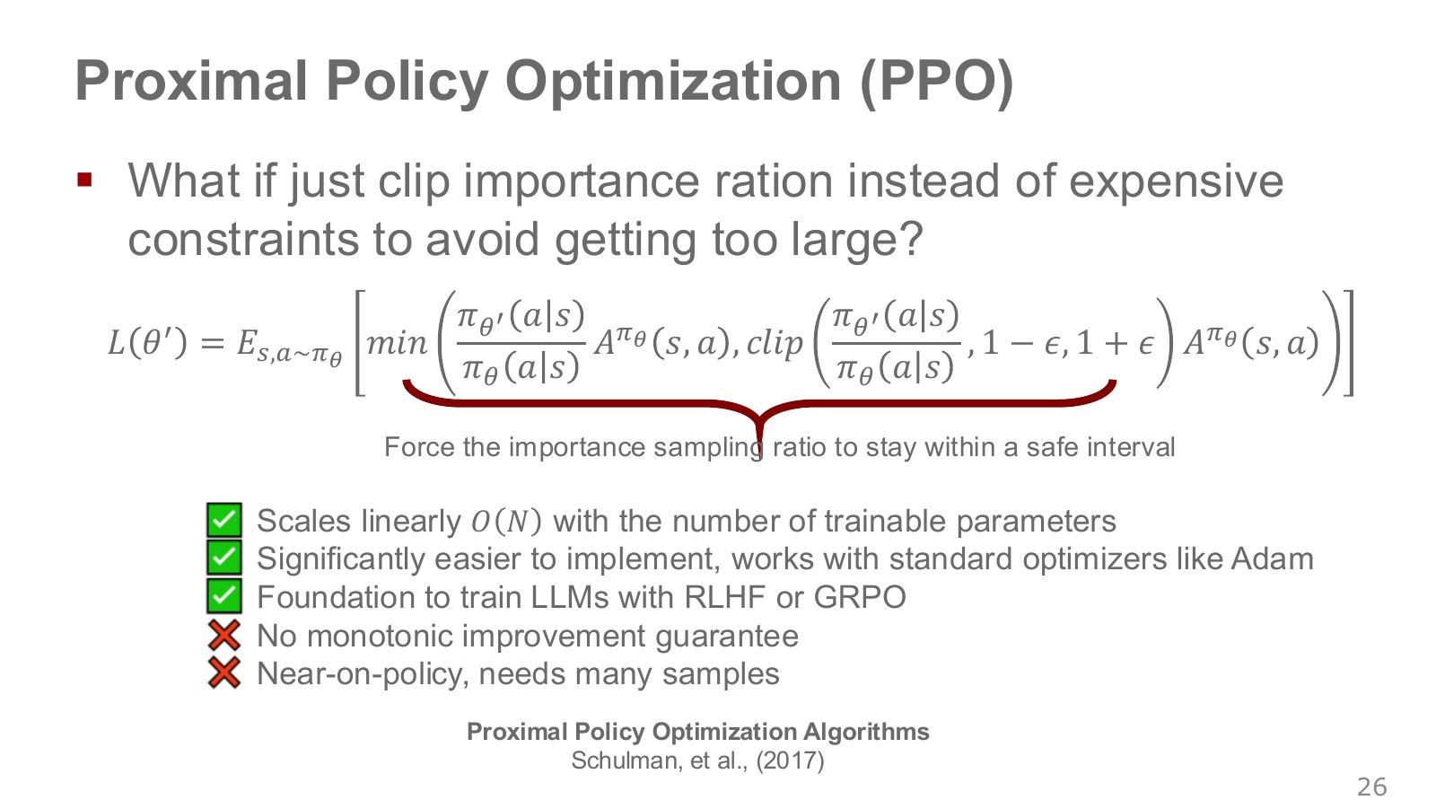
Instead of complex KL-constrained optimization, PPO-Clip clips an objective formed from probability ratios and advantages. The ratio divides the new action probability by its probability during collection. With set to 0.2, the clipped ratio lies between 0.8 and 1.2.
Explore the symbols and calculation The PPO clipped surrogate objective
Read the equation in words
Use the more conservative of the original value and a value limiting gains from policy change. This cuts off incentives to increase favorable actions or decrease unfavorable actions excessively.
Understand each symbol
- New-policy action probability divided by old-policy probability. In this equation, it is not a motor input.
- An estimated advantage indicating how much better this action is than the state's average.
- The parameters collecting the trainable weights of the network or policy.
- The ratio-clipping tolerance, usually a small positive number.
- Restrict a comparison ratio to an allowed interval. This does not guarantee that the policy itself remains inside that interval.
- An expectation: an average over possible outcomes weighted by their probabilities.
Follow the calculation
- Also calculate the probability ratio clipped to the allowed interval.
- Multiply the original and clipped ratios by advantage and select the smaller score.
Check with a small example
With advantage 2, ratio 1.5, and tolerance 0.2, the score is . For negative advantages, include the sign when deciding which term is smaller.
An illustrative example for understanding the equation.
With advantage +2, ratio 1.5 gives an unclipped objective of 3, but the clipped term is 2.4, so the smaller value 2.4 is used. Once a good action has been increased sufficiently, that sample provides no further incentive to increase it. Conversely, with advantage −2 and ratio 0.5, the clipped term −1.6 is smaller than the original term −1, so −1.6 is used. This cuts off additional gains after a bad action has already been reduced sufficiently.
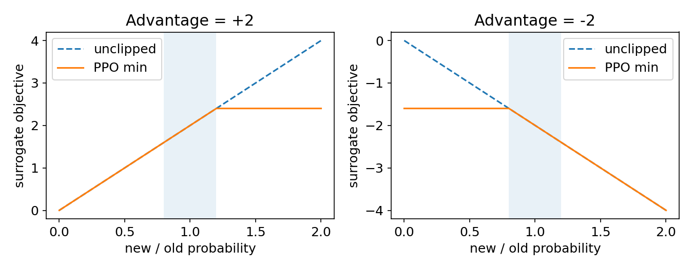
The policy’s actual ratio is not forcibly kept inside the interval. Changes in an unfavorable direction retain an unclipped penalty, and updates from other samples through shared weights can move this sample’s ratio farther. PPO does not inherit TRPO’s theoretical monotonic-improvement guarantee. Some implementations also monitor KL or stop updates early. Its ease of use with first-order optimizers such as Adam is a major advantage.
Related objectives also appear in language-model training, but GRPO and PPO should not be called the same algorithm. This chapter focuses on robot-policy data collection and continuous control.
#P028 · Rubik's Cube manipulation combines control, state estimation, and simulation
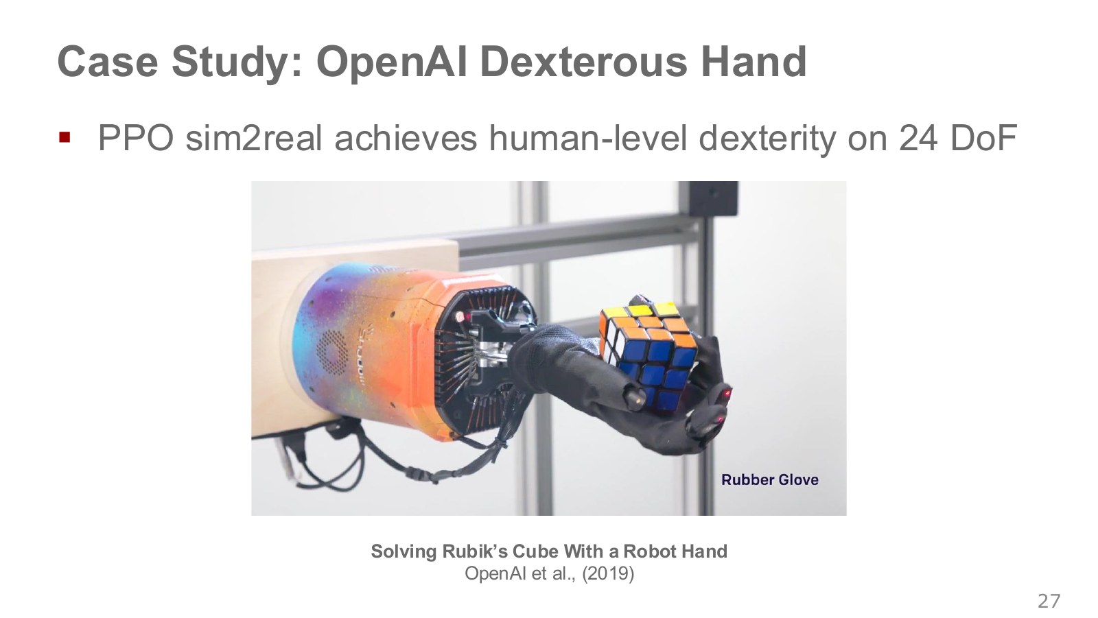
The five-fingered robot hand in the photograph reorients a cube and turns its faces while maintaining its grasp. Familiar to humans, this manipulation is a difficult control problem involving changing contacts and possible object slippage. The rubber glove illustrates a perturbation to friction and contact conditions.
OpenAI’s 2019 research used a recurrent control policy trained with PPO and a separate vision model estimating cube pose and face rotations from camera images. It should not be read as feeding raw camera images directly into the final manipulation policy to solve every part jointly. Also distinguish planning the high-level cube-solving sequence from physically executing the next manipulation target with the hand.
Automatic domain randomization (ADR) progressively broadens the physical and visual conditions encountered in simulation. This encourages operation under varied conditions rather than fitting only one simulator’s friction or appearance. The photograph does not demonstrate every form of human-level dexterity; it shows results for the cube task and perturbations defined in the paper. Hardware degrees of freedom and the number of independently commanded actuators are not always identical either.
The lecture’s video with some fingers tied together illustrates policy robustness when familiar manipulation conditions change. Even rotating an object in the same direction becomes difficult to accomplish by replaying the old trajectory if available fingers and contacts change. ADR varies physical conditions during training to broaden experience with such differences. Read the demonstration alongside the actual altered conditions and successful tasks, rather than extending it into a recovery guarantee for every finger failure or object.
#P029 · PPO's full objective combines the actor, critic, and exploration
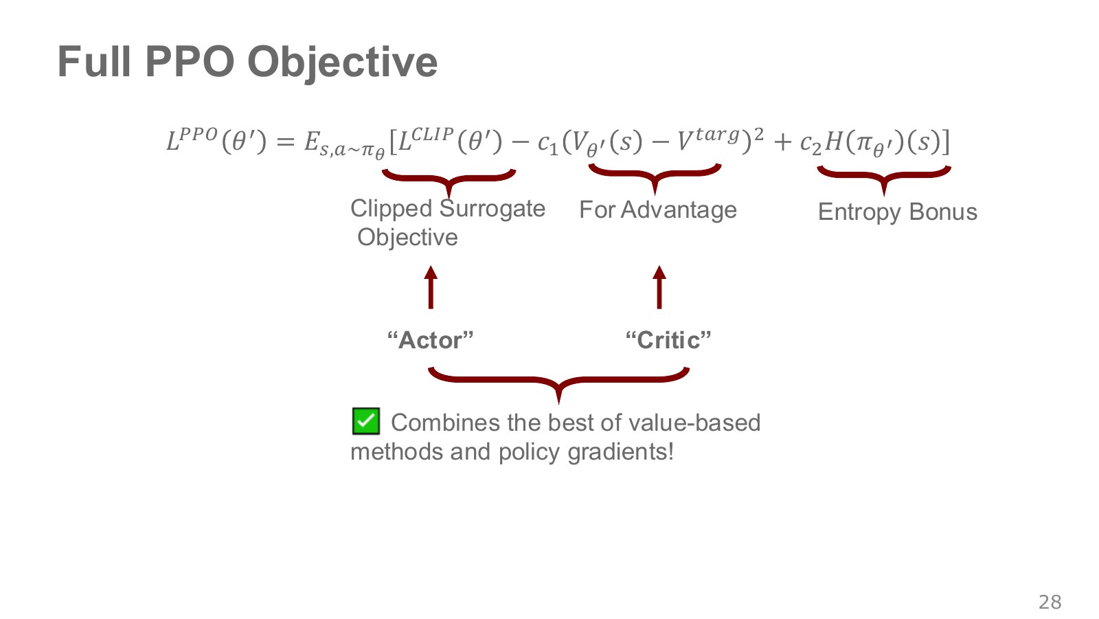
The first term is the clipped surrogate objective encouraging the actor to increase good actions’ probabilities. The second is squared error fitting the critic’s state value to a target return. The third is an entropy bonus discouraging the policy from concentrating too quickly on one action.
Explore the symbols and calculation The full PPO maximization objective
Read the equation in words
Combine increasing good actions, reducing value-prediction error, and maintaining exploration. The signs here define an objective to maximize.
Understand each symbol
- The parameters collecting the trainable weights of the network or policy.
- The current value prediction and the value target it should match.
- Relative weights for the value loss and entropy term.
- An expectation: an average over possible outcomes weighted by their probabilities.
- Conditional notation: the information to the right of the bar is given. This is not a division sign.
Follow the calculation
- Subtract weighted squared value-prediction error from the policy surrogate objective.
- Add weighted policy entropy. Converting to minimization code requires adjusting the overall signs consistently.
Check with a small example
With policy score 1, value loss 0.4 weighted by 0.5, and entropy 0.6 weighted by 0.01, the total score is 0.806.
An illustrative example for understanding the equation.
Because the expression is maximized, value error carries a minus sign. In a loss to be minimized, reverse the first and third terms’ signs and keep value error positive. The coefficients and balance terms with different units.
The quantity is the target the critic attempts to fit. Its construction varies by implementation, using complete observed returns, bootstrapped returns, or other choices. Store the actor’s advantage estimates separately from critic targets, and usually hold advantages fixed during actor updates. When the networks share an initial representation, gradients from all three terms change it together, so clipping a single sample does not strictly constrain overall policy change.
#P030 · Actor–critic learns action selection and future evaluation together
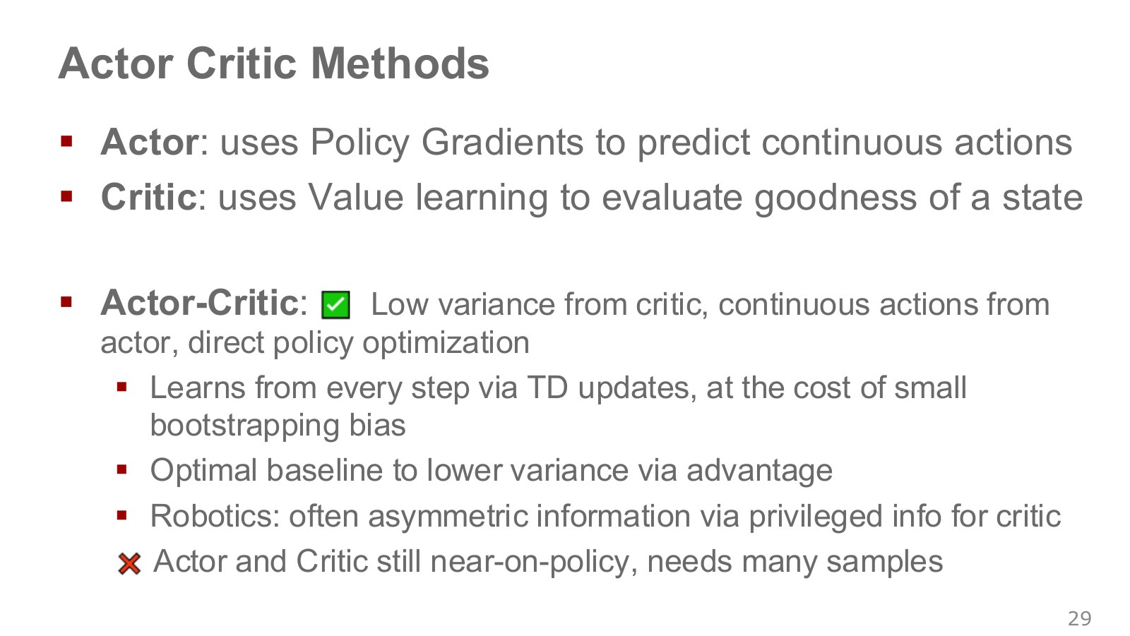
The actor is the policy, and the critic is a value estimator. The actor uses whether outcomes exceeded the critic’s expectations as a signal for changing action probabilities. Actor–critic is not restricted to continuous actions; it also applies to discrete-action policies. Nor is every actor–critic method on-policy, as the contrast between PPO and SAC demonstrates.
Giving a critic object positions available only in simulation can improve value estimation during training. The deployed actor can be restricted to actual cameras and sensors. Record critic and actor inputs separately to make clear which information is required on the real robot.
The simplest advantage estimate based on a one-step TD error is:
Explore the symbols and calculation TD error accounting for termination
Read the equation in words
The difference between the current value prediction and a target reconstructed from a one-step observation. A termination indicator removes value after an actual terminal transition.
Understand each symbol
- The TD error: the difference between the one-step target and the current value estimate.
- The reward received at one step: a learning signal defined so that larger is better.
- The discount factor for future rewards. Zero considers only the immediate reward, while values near one give more weight to the distant future.
- An indicator equal to 1 for actual termination and 0 otherwise. It prevents adding future value after termination.
- The critic's predicted state value.
Follow the calculation
- Add discounted next-state value to the immediate reward.
- Subtract current-state value to obtain the error. Remove the future term on termination.
Check with a small example
Reward 1, next value 4, discount factor 0.9, and current value 3 give error 1.6. On termination, it is .
An illustrative example for understanding the equation.
The indicator is 1 on actual termination. If the critic is accurate and the state contains sufficient information, this error indicates the action’s relative value. An inaccurate critic does not automatically yield low bias. Future value is zero when an episode truly ends, whereas a rollout cut short merely by collection length requires appropriate bootstrapping.
Generalized Advantage Estimation (GAE) combines multistep TD errors, using to balance short-term bootstrapping against longer sampled returns. With it becomes one-step TD; summing over longer horizons brings it closer to sampled returns. This controls the trade-off between variance and value-approximation error. The original GAE paper is useful background before reading a PPO implementation.
Robot simulation can also use an asymmetric setup where only the critic sees additional information, such as true terrain friction or exact object state. The deployed actor must still operate from real sensors, and not every use of privileged information satisfies the same statistical conditions.
#P031 · SAC evaluates current-policy actions at past states
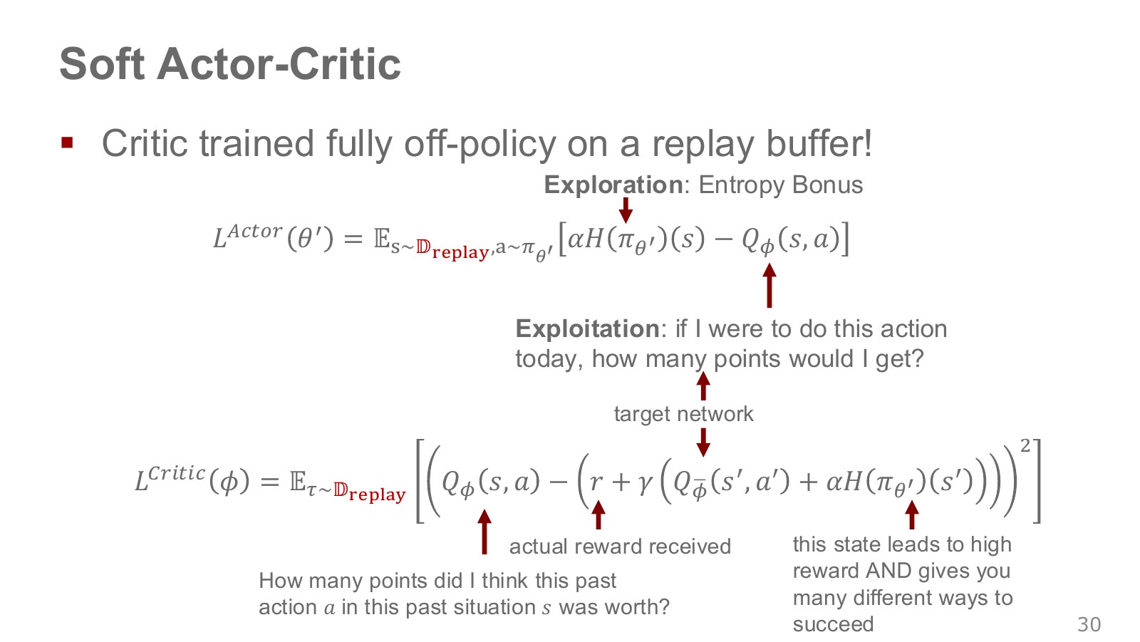
SAC trains its critic on past transitions from a replay buffer. Actor updates also use past states, but draw fresh actions at those states from the current policy. This differs from learning to reproduce the old actions stored in the buffer. The critic estimates the value of these current actions and supplies the actor’s learning signal.
SAC uses a maximum-entropy reinforcement-learning objective that increases policy entropy as well as reward. The actor’s maximization objective combines expected and entropy. Converting it into a minimization loss gives the following signs.
Explore the symbols and calculation The SAC actor loss to be minimized
Read the equation in words
The SAC actor minimizes a loss favoring both high value and sufficient randomness. It uses the smaller evaluation from two critics.
Understand each symbol
- The parameters collecting the trainable weights of the network or policy.
- SAC's entropy weight or temperature. Here, it is not a learning rate.
- Replay data storing transitions for later sampling.
- Action-value estimates from two different critics.
- An expectation: an average over possible outcomes weighted by their probabilities.
- The natural logarithm. It converts products into sums and is defined only for positive inputs.
- Conditional notation: the information to the right of the bar is given. This is not a division sign.
Follow the calculation
- Sample an action from the current policy and evaluate it with both critics.
- Minimize the average of the log action-density term minus the smaller value estimate.
Check with a small example
With log density −1, temperature 0.2, and values 3 and 4, the sample loss is . Remember the minimization convention: lower is better.
An illustrative example for understanding the equation.
Because entropy is the negative expected log probability, minimizing corresponds to maximizing . Minimizing the slide’s actor expression unchanged would instead reduce entropy, so the main text explicitly uses the original paper’s log-probability form to clarify the sign.
In the equations below, theta denotes actor weights and phi critic weights. The subscript identifies which of the two critics is meant, and a bar over phi denotes a target copy. The symbol denotes the replay buffer of past transitions. Practical continuous-action SAC uses two estimators and slowly updated target copies. A current-policy action sampled at the next state forms the target below; each critic reduces its squared error against that target.
Explore the symbols and calculation The SAC soft TD target
Read the equation in words
SAC's TD target includes the next action's entropy contribution along with next-state value. Like the actor loss, it uses the minimum critic value.
Understand each symbol
- The reward received at one step: a learning signal defined so that larger is better.
- The discount factor for future rewards. Zero considers only the immediate reward, while values near one give more weight to the distant future.
- An indicator equal to 1 for actual termination and 0 otherwise. It prevents adding future value after termination.
- A target critic updated more slowly than the critic being trained.
- The entropy temperature and an action freshly sampled at the next state.
- The natural logarithm. It converts products into sums and is defined only for positive inputs.
- Conditional notation: the information to the right of the bar is given. This is not a division sign.
Follow the calculation
- Sample a current-policy action at the next state.
- Subtract temperature times log density from the smaller target-critic value, discount the result, and add the reward.
Check with a small example
If the smaller target value is 4, log density is −1, and temperature is 0.2, the bracket equals 4.2. Reward 1 and discount factor 0.9 give target 4.78.
An illustrative example for understanding the equation.
Using the smaller estimate helps mitigate overestimation. The temperature determines the relative importance of entropy and reward. Changing reward scale also changes an appropriate temperature. Automatic temperature tuning learns this coefficient against a target entropy; it does not enforce identical randomness in every state. The update equations were also checked against SAC Algorithms and Applications.
#P032 · Reparameterization constructs an action from fixed noise and differentiates that path
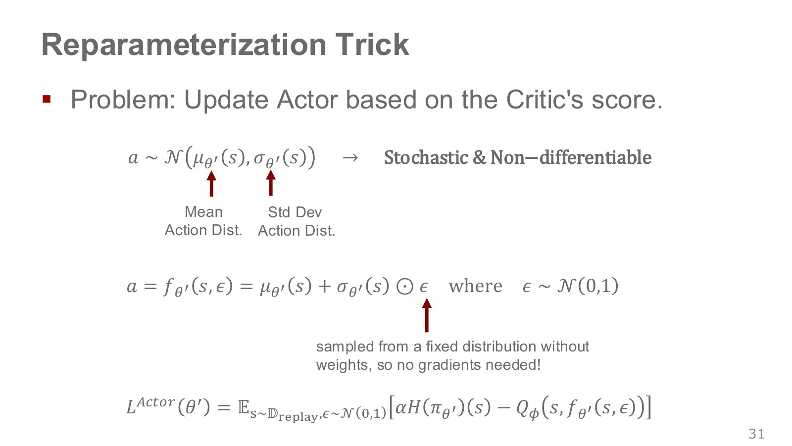
When a policy outputs a mean and standard deviation, treating an action simply as a sampled value does not preserve its connection to those parameters in the autodifferentiation graph. Instead, first sample standard-normal noise independent of the parameters, then combine it with the policy outputs to construct the action.
Explore the symbols and calculation Gaussian reparameterization
Read the equation in words
Instead of sampling the Gaussian action directly, sample standard noise and transform it using the mean and standard deviation. This transformation connects changes in the output action to changes in weights.
Understand each symbol
- Sample a Gaussian noise vector with component means 0 and variances 1.
- The Gaussian action sample before tanh bounds its range. This differs from PPO's probability ratio.
- The mean and standard deviation predicted by the policy.
- Elementwise multiplication of corresponding vector components.
Follow the calculation
- The policy predicts a mean and positive standard deviation from the state.
- Multiply standard noise by standard deviation elementwise and add the mean.
Check with a small example
Mean 0.2, standard deviation 0.1, and noise −0.5 give a presquash action of 0.15.
An illustrative example for understanding the equation.
Holding fixed for this sample makes the path from mean and standard deviation to action differentiable. The symbol means elementwise multiplication. This path passes the critic’s action derivative to the actor. Unlike REINFORCE’s log-probability derivative, this approach uses a differentiable critic and continuous action-generation function. It does not backpropagate through real-world contact.
When commands have bounded ranges, policies often squash Gaussian samples as in . The action log density then requires a Jacobian correction for the coordinate transformation.
Explore the symbols and calculation The tanh log-density correction
Read the equation in words
Squashing a Gaussian sample through tanh bounds the action but also changes its probability density. A log correction accounts for stretching or compression under the coordinate transformation.
Understand each symbol
- The actual action, bounded between −1 and 1.
- The density of the Gaussian sample before transformation.
- The derivative of tanh. Numerically stable computation is needed near the boundaries.
- Add every term over the indicated range, computing one term and repeating through the end of the range.
- The natural logarithm. It converts products into sums and is defined only for positive inputs.
- Conditional notation: the information to the right of the bar is given. This is not a division sign.
Follow the calculation
- Calculate the Gaussian log density of the presquash sample.
- Subtract the sum of log elementwise tanh derivatives to obtain the actual action's log density.
Check with a small example
A presquash value of 0 has derivative 1, so its correction is zero. At 1, the derivative is approximately 0.42 and the log correction has a larger effect.
An illustrative example for understanding the equation.
Simply clipping actions while retaining the original Gaussian log density in the entropy term gives a distribution mismatch. Numerical stability near saturation also needs checking. The example below compares a reparameterized sample’s derivative with finite differences and separately checks numerical values for the tanh density correction.
#P033 · Read real-robot results alongside both the algorithm and experimental conditions
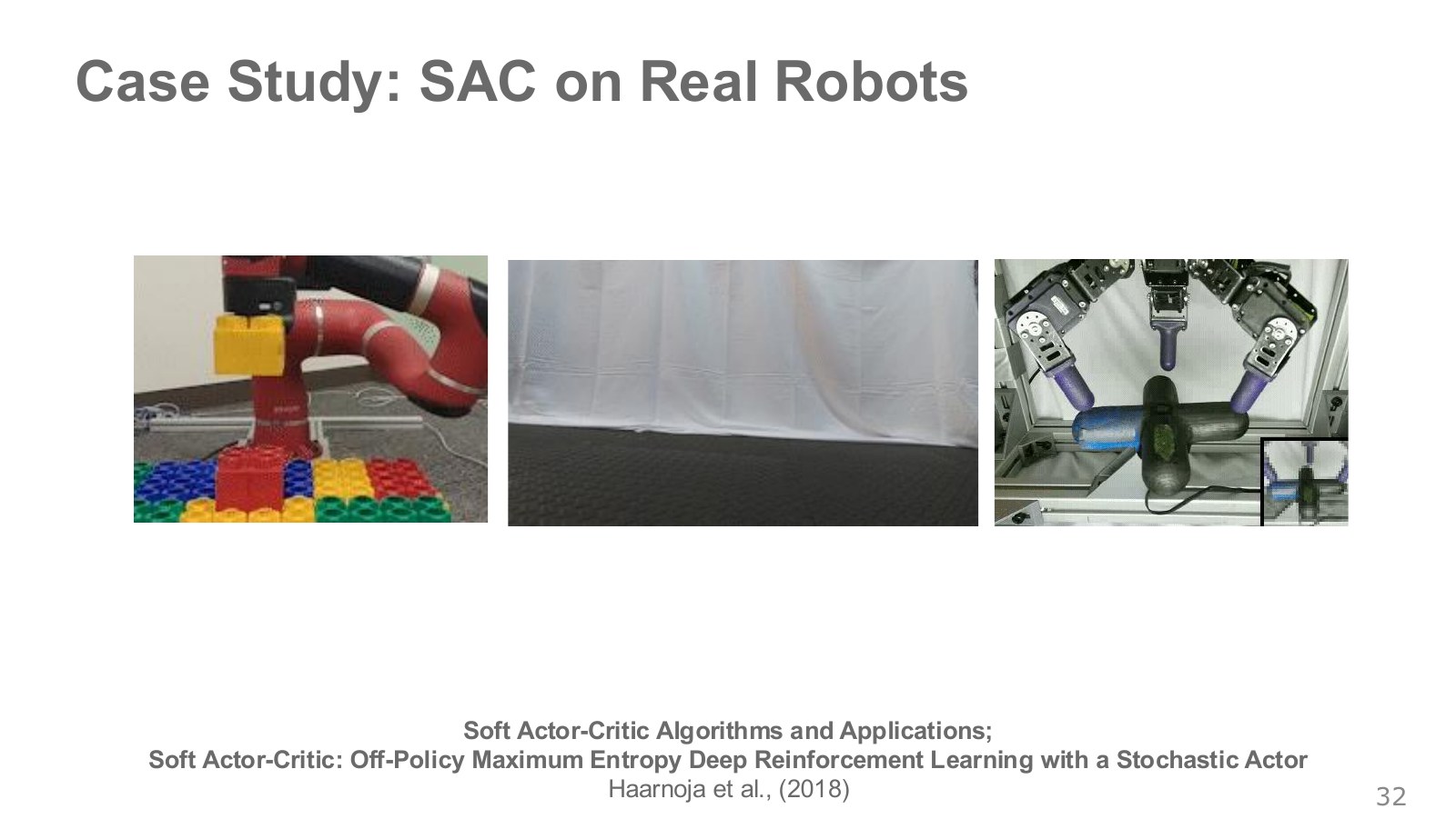
The three photographs illustrate different contact problems: manipulating objects, quadruped locomotion, and reorienting an object within a hand. Understanding each result requires knowing its observations, action space, reward design, reset procedure, and hardware conditions.
The original SAC paper and subsequent Applications paper combine replay buffers, a stochastic actor, and an entropy objective to evaluate data efficiency and stability in continuous control. They also present real quadruped locomotion and hand manipulation. We should not assume that every photograph assembled on the slides comes from one experiment or the same SAC version. A still image alone also cannot reveal a video’s sequence or failure rate.
Replay buffers do not eliminate collection costs. An overly optimistic critic in a new state–action region can be exploited by the actor. Evaluations favoring SAC’s data efficiency do not establish that it always outperforms PPO on every robot task. This chapter’s small executable examples likewise do not reproduce those robot experiments.
#P034 · Distinguishing policy gradients, PPO, and SAC by their data and objectives
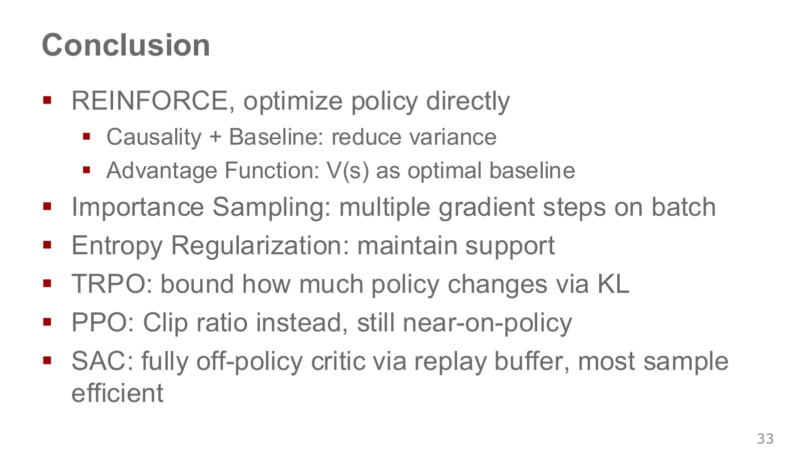
REINFORCE weights action log probabilities using outcomes generated by the current policy. Reward-to-go removes past rewards; a baseline subtracts a reference independent of the current action; advantage compares against the current state’s expected average. Their shared aim is a more accurate, less noisy signal for policy improvement.
TRPO and PPO control policy change to keep improvement estimates from the previous batch useful. PPO trains several times on a recent batch but does not reuse old data without limit. SAC learns from past transitions, asks the critic about freshly sampled current-policy actions, and optimizes an objective that includes entropy.
| Method | Signal used by the actor | What matters about data use |
|---|---|---|
| REINFORCE | Sampled return × log-probability gradient | Runs generated by the current policy |
| PPO | Fixed advantages and a clipped probability-ratio objective | Limited repeated updates on a recent batch |
| SAC | Soft and log probability for current-policy actions | Replay of past transitions; fresh current-action samples |
For any algorithm, the meanings of state, action, and reward come first. Likewise, read reported success rates alongside observations, hardware, training-data volume, and evaluation conditions. The code below shows how this chapter’s key equations differ numerically.
#Calculations run and checked for this article
The example code, execution instructions, and result CSVs are available. The examples run REINFORCE on a one-state, two-action problem and check baseline variance, importance-weighted averages, all four directional cases of the PPO objective, SAC targets, and reparameterization derivatives. They are not results from training a robot simulator or PPO/SAC neural networks.
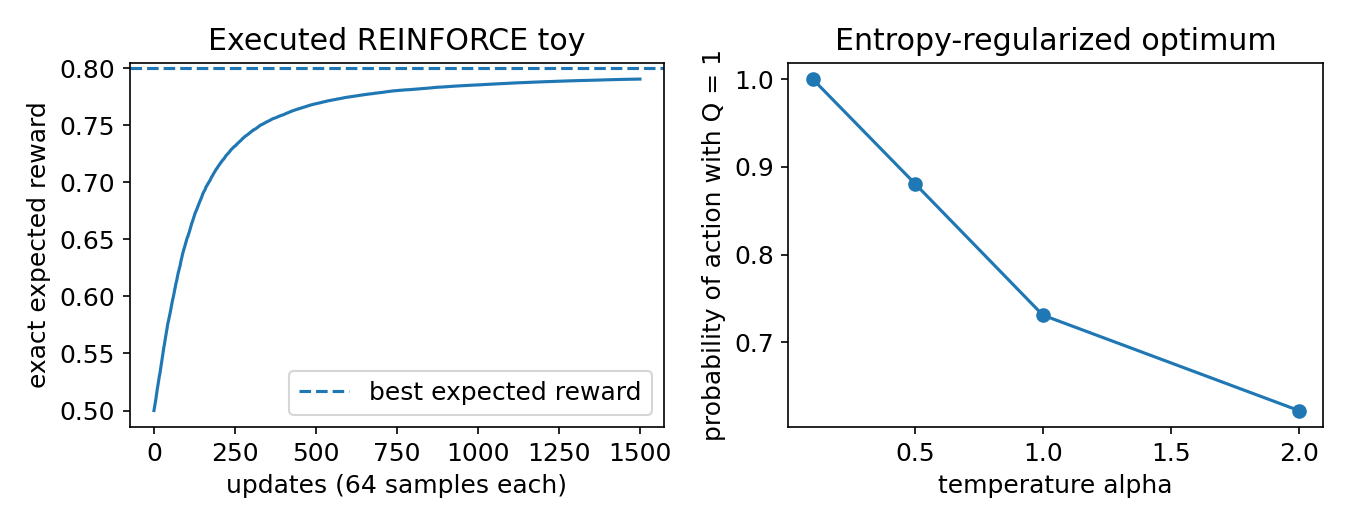
For selection probability 0.3 and returns 99 and 101, the exact policy gradient was 0.42. The baseline is 99.6, while the variance-minimizing baseline for this problem is 100.4. Subtracting the same-batch mean with =2 reduces the expected gradient to 0.21, while a leave-one-out baseline preserves 0.42. This illustrates why “subtracting a baseline is always unbiased” must be read together with implementation conditions.
In the SAC target calculation, reward 0.2, discount factor 0.9, next Q value 1.5, temperature 0.2, and log probability −0.7 yield a target of 1.676. On actual termination, removing the future term leaves 0.2. These numbers check algorithmic signs and termination handling, rather than real-robot performance.
#Sources and further reading
- ETH Robot Learning 2026: Lecture 5 slides were compared with the technical portion of the public recording, 0:00–52:20.
- David Silver, Lecture 7 slides and public recording: additional connections between score functions, REINFORCE, actor–critic, and baselines.
- Berkeley CS285 2023 materials: topic-by-topic comparisons with Lecture 5 on policy gradients, Lecture 6 on actor–critic, and Lecture 9 on advanced policy gradients.
- Original TRPO paper, original PPO paper, and original GAE paper: references for distinguishing theoretical guarantees from practical approximations, and clipping objectives from value targets.
- Initial SAC paper and SAC Algorithms and Applications: references for entropy objectives, replay buffers, twin estimators, temperature adjustment, and reparameterization.
- Quadruped locomotion over challenging terrain and Rubik’s Cube robot hand: conditions for connecting simulation with real robots.
Rights to the original slides belong to Oier Mees and the respective original authors and rights holders. Figures in the article use a pinned public copy. JJo created the explanatory text and calculation plots. The page, caption, and source comparison record documents provenance and review coverage for each resource.