To grasp a cup, a robot benefits from anticipating an action’s consequences before moving its arm. If Chapter 7 explained reading observations and commands in sequence, this chapter explores testing the future with commands not yet executed.
Copyright in the slides belongs to Oier Mees and the original rights holders of each figure and video. Numbers follow PDF page order. The explanation was checked against the lecture’s automatic captions, skipping administrative announcements to organize the technical content. Video links below slides jump to the relevant explanation. Official ETH Zurich course · Official PDF · Lecture 8 video
#Project announcements at the start of the lecture
Before defining world models, Lecture 8 introduces five team projects using student-assembled SO-101 robots. Responding to feedback that paper discussions move too quickly, the lecturer proposes shifting some presentations to Thursday and allowing more lecture time. Demo dates and H100-resource announcements concern students enrolled at that time. The overview below focuses on which models the projects aimed to test and how. Project announcements
| Project | Initial task | Increasing difficulty | Bonus evaluation |
|---|---|---|---|
| VLA | Pick and place a plastic banana | Instructions requiring left–right relations and understanding unfamiliar pictures | Perform with a small model |
| World model | Push an object in a straight line | Push around obstacles to a goal; introduce unfamiliar objects | Reach the goal in fewer actions |
| Reinforcement learning | Start from a policy placing a block in a bowl | Separate four clustered blocks, then extend to more blocks | Faster separation |
| Typing | Move the fingertip among four points on paper | Press specified keys, then type words on another keyboard | Faster typing |
| Clothes folding | Grasp an edge and make one fold | Extend to consecutive folds and folding an entire garment | Complete folding and speed |
The lecturer explains that the initial policy for block separation can be built through behavior cloning. Distinguish a project’s name from the learning method used at each stage. Typing can use a key-pressing tool attached to the gripper, while an unfamiliar keyboard must still fit within the arm’s workspace. Clothes folding applies the diffusion policies studied in class to deformable objects.
#What should an action-conditioned model predict?
#P010 · Can a robot anticipate consequences before acting?
Suppose a robot pushes a cup onto a plate. A command alone cannot reveal whether moving the hand another centimeter will settle the cup on the plate or catch the rim and tip it over. A world model predicts what follows from observations so far and proposed actions. These predictions can support both candidate-action selection and policy training.
The SO-101 projects introduced before the technical lecture illustrate how to test a world model. Difficulty increases from straight pushing to moving around obstacles and handling unfamiliar objects. Even when the model predicts motion, reaching the goal and the number of actions used are evaluated through actual execution. Project introduction
#P011 · A batter anticipates where the ball will arrive
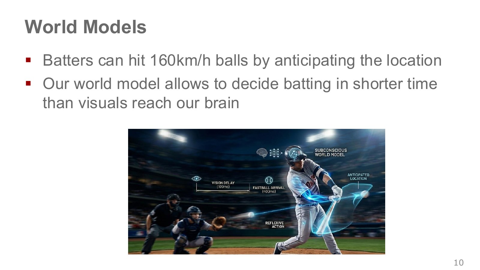
Time separates the ball’s illustrated position from the bat’s future position. A batter estimates direction and speed from a few observations and allows time to swing. Likewise, a robot may need different commands for a ball at the same image location depending on whether it arrives from the left or right.
Using the lecture’s approximate figures, ball travel takes about 400 ms and visual-signal transmission about 100 ms, leaving roughly 300 ms for judgment and swinging. These are lecture approximations. They explain why a batter anticipates arrival from the early trajectory rather than waiting to react after the ball reaches the plate.
#P012 · A policy chooses an action; a world model predicts its outcome
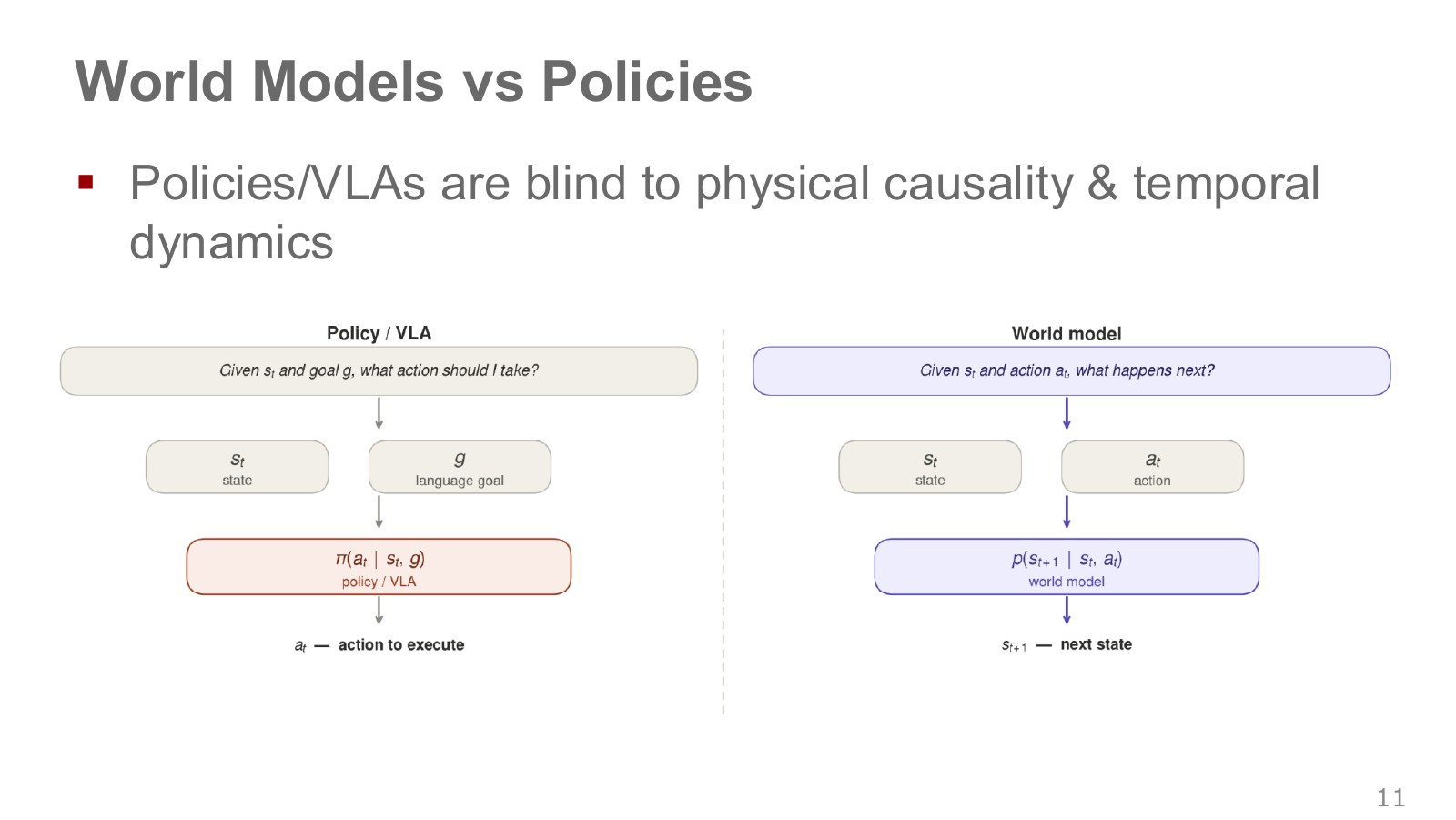
The left arrow maps a current state and goal to an action: given “move the cup onto the plate,” the policy chooses a hand-motion direction. The right maps a current state and candidate action to a next state. Left and right pushes can be supplied separately to compare outcomes for the same cup. A VLA using image history may also learn motion regularities. The distinction here concerns the inputs and outputs provided externally.
Explore the symbols and calculation Questions posed to policies and world models
Read the equation in words
The left asks which action to choose for a goal; the right asks what happens next when an action is specified.
Understand each symbol
- Current state
- Goal
- Action to choose now
- State after acting
Follow the calculation
- Suppose the cup is left of the plate. Given a goal of moving it onto the plate, a policy may choose a rightward push.
- Supply that push to the world model to predict the cup's next position or chance of tipping.
Check with a small example
A policy assigning probability 0.8 to a rightward push does not imply success probability 0.8. Success must be evaluated from predicted outcomes separately.
An illustrative example for understanding the equation.
#P013 · Test several plans from the same starting point
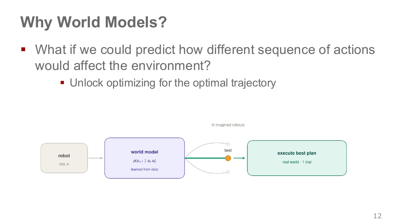
Each branch from the central box is a predicted trajectory, or rollout, formed by connecting several actions. An easy first move can still lead to a poor overall plan if the cup later meets a wall. A longer initial detour to the right may be worthwhile if it reaches the final goal. After actual execution, a fresh observation updates the starting point.
#P014 · Physics engines and simulators learned from data
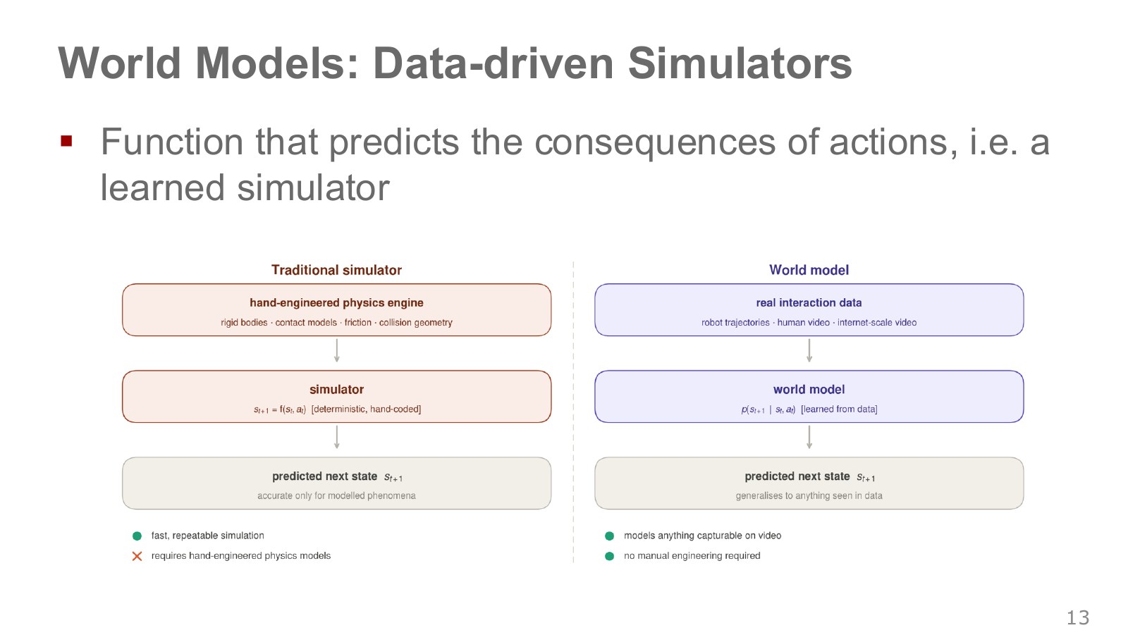
The simulator on the left computes next states from specified masses, friction, and contact rules. The model on the right estimates transition patterns from experience pairing observations with robot commands. It can learn difficult-to-model scenes such as folding cloth, but may predict unfamiliar materials or contacts incorrectly. The approaches can also be combined.
If a rigid box’s mass and friction are known, a physics engine can quickly test different pushes. Specifying every contact and material interaction becomes harder for wet cloth folding or soft tissue deforming under pressure. A learned model can acquire such changes from image–action pairs, but may also need substantial data to relearn simple motion laws already known analytically. The lecture’s choice depends on the phenomena to represent and the available experience.
#P015 · The next state may be one prediction or a distribution of outcomes
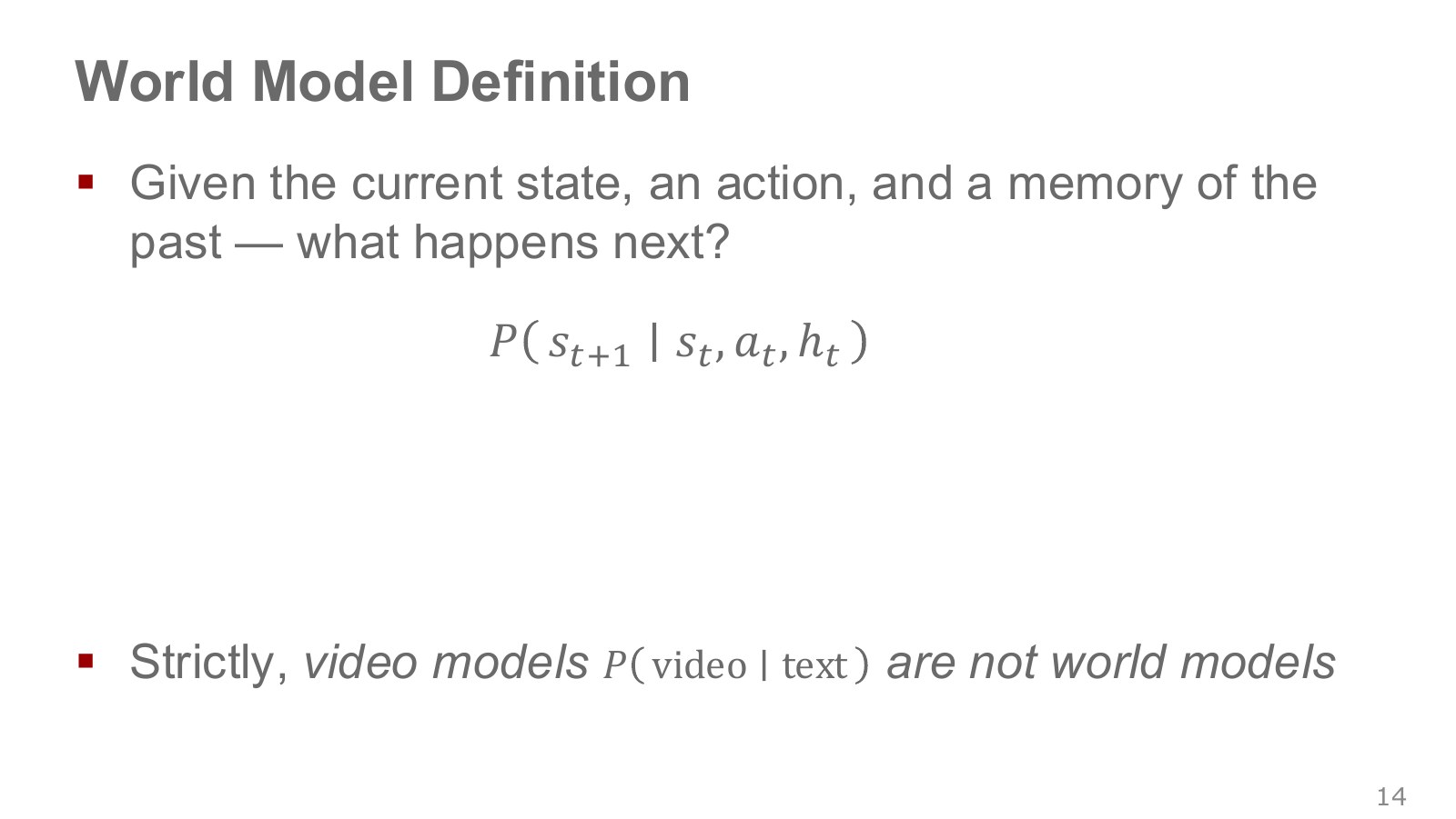
A cup pushed at the same speed may slide farther on a wet surface. A conditional distribution describes which outcomes are plausible given current knowledge. The lecture’s action-conditioned world models accept concrete candidate actions when predicting the future. A text-conditioned video model does not inherently provide this action input.
Explore the symbols and calculation Transitions conditioned on current state, action, and memory
Read the equation in words
Terms right of the vertical bar are information already given; the left is the unknown next state to predict.
Understand each symbol
- Memory from the past
- Current state or estimate
- Command to test
- Transition distribution learned from data
Follow the calculation
- Fix the current cup position and a command to push right.
- Adding memory of earlier slipping on the surface can increase the predicted likelihood of farther movement.
Check with a small example
If only two nonoverlapping positions are possible and the nearer receives probability 0.7, the farther receives 0.3.
An illustrative example for understanding the equation.
#Planning through video
#P016 · Predict movement rather than repainting every pixel
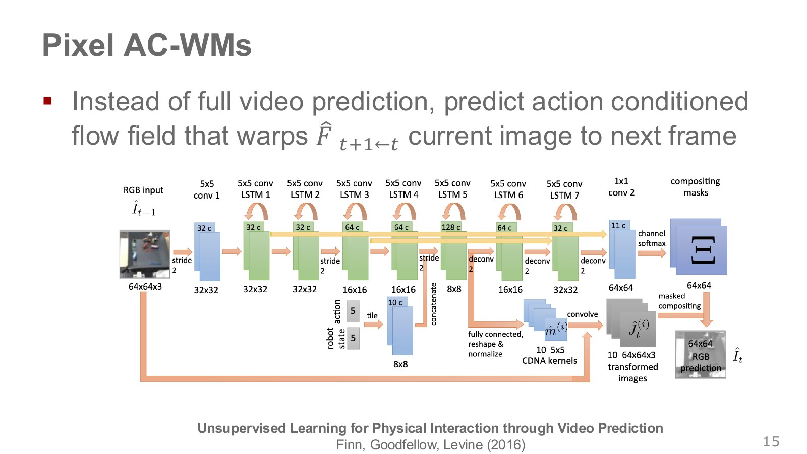
The left camera frame propagates along the orange path toward the right. Finn and colleagues’ CDNA model applies multiple transformations to previous images and uses masks to mix them across regions. The robot arm and cup can move differently while the background remains fixed. Motion alone cannot easily reveal the color and shape of newly exposed surfaces absent from the previous frame. Finn et al., Video Prediction
When a cup moves rightward, predicting where existing pixels go makes it easier to preserve wall patterns and table colors than redrawing them every time. Early convolutional LSTMs read spatial features while remembering motion across frames. Multiple transformations and occlusion handling help address newly visible regions. This motion-centered structure helped learn future video from the relatively limited interaction data available then. Finn et al., action-conditioned video prediction
#P017 · A point selected on an image becomes the robot's goal
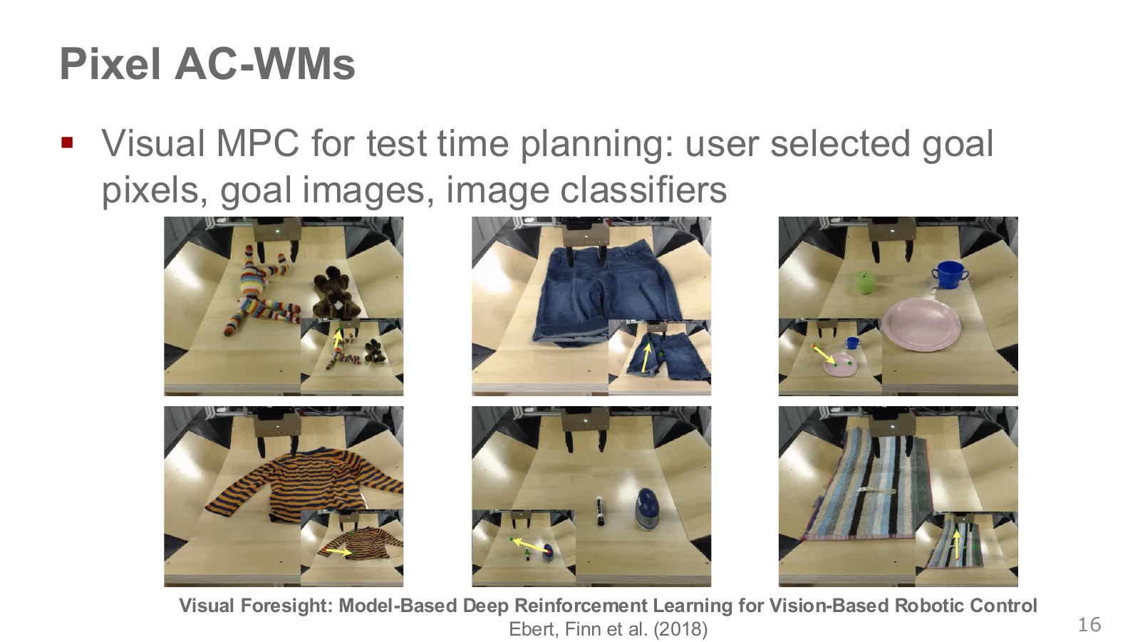
As in the cloth and plate examples, users can select an image point to move and its destination. Candidate predictions receive lower cost when that point approaches the target. Alternatively, users can supply a desired final image or a classifier score for “drawer closed.” Different definitions of success allow the same world model to plan different tasks. Ebert et al., Visual Foresight
Visual Foresight trains on interaction videos and actual commands collected autonomously by a robot. Predicting next images does not require human task labels such as “move this object there.” At execution, the user selects goal pixels to rank candidate paths.
#P018 · CEM narrows candidates; MPC checks again after execution
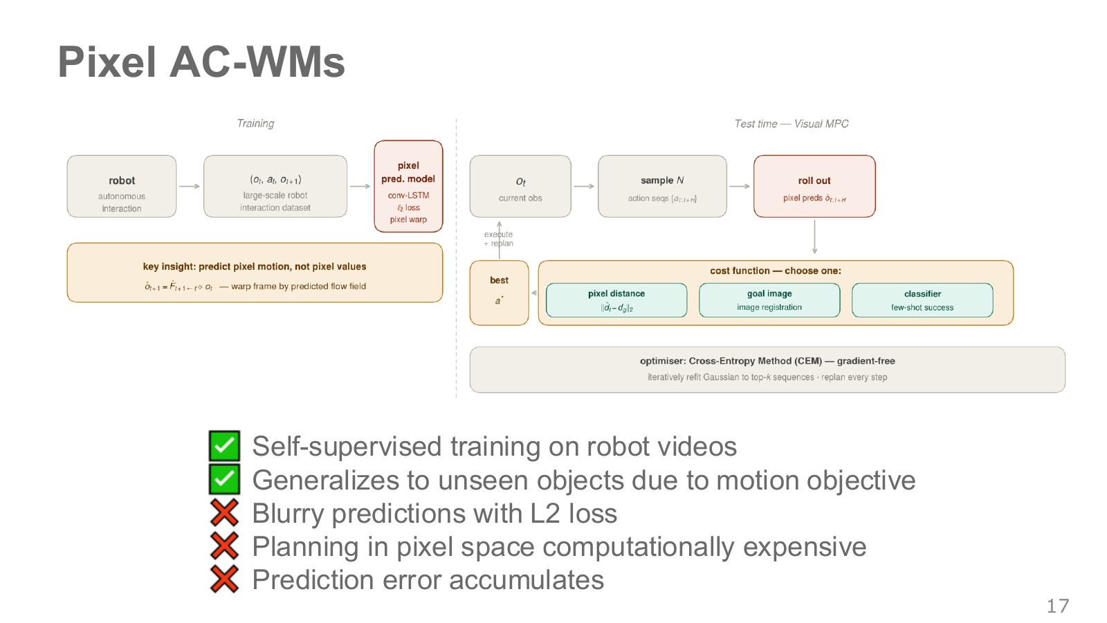
The left side shows model training: collect commands and before-and-after images, using the next frame as a target. The right shows execution. The Cross-Entropy Method (CEM) samples action sequences, selects low-predicted-cost elites, and updates the next sampling distribution. Model Predictive Control (MPC) executes only the beginning of the selected sequence, observes the real scene, and replans. CEM searches for candidates; MPC revises plans through observations during execution.
Pixelwise squared error can blur object outlines by averaging two possible locations. Feeding predicted frames into subsequent predictions accumulates mismatch. Computing many frames for every candidate adds cost, motivating later latent-space methods that compress control-relevant information for comparison.
Berkeley CS285 explains that replanning every few steps reduces reliance on each plan’s accuracy and allows shorter horizons. If a cup slides less than expected after the first move, the remaining commands can be recalculated from its observed position. Sergey Levine, CS285 model-based reinforcement-learning slides
Explore the symbols and calculation Selecting the action sequence with low predicted cost
Read the equation in words
Predict successive future states for each candidate action sequence and select the sequence with the smallest total state cost.
Understand each symbol
- Prediction horizon
- Candidate action sequence
- Cost measuring factors such as distance from the goal
- Model-predicted state
Follow the calculation
- Start two candidate rollouts from the same actual observation and predict two steps for each.
- Sum each candidate's costs and execute the better candidate's first action. Replan when new sensor readings arrive.
Check with a small example
Two candidates with step costs [3,1] and [2,1] have total costs 4 and 3. Select the second within this candidate set.
An illustrative example for understanding the equation.
Follow the planning procedure: the user selects a point on the cup and a target point. The planner samples several multistep arm-motion sequences and predicts the images each would produce. It retains candidates approaching the target pixel and adjusts the next candidate distribution. This repetition is CEM. Executing only the beginning of a good sequence and restarting from a new photograph is MPC.
If weak contact moves the cup less than expected, the next photograph captures the discrepancy. Executing the entire original long sequence would instead continue commanding against a mistaken cup position. This is why actual observations are incorporated repeatedly. Visual Foresight
#Imagining in latent space
#P019 · Must every prediction redraw the entire screen?
More candidates and longer horizons increase the cost of repeatedly generating full images. A short numerical vector can instead retain information important for action selection, such as cup position and motion. This compressed representation is a latent representation. If compression removes whether the cup is grasped, fast computation can still select a poor plan.
#P020 · Practicing policies in a compressed state space
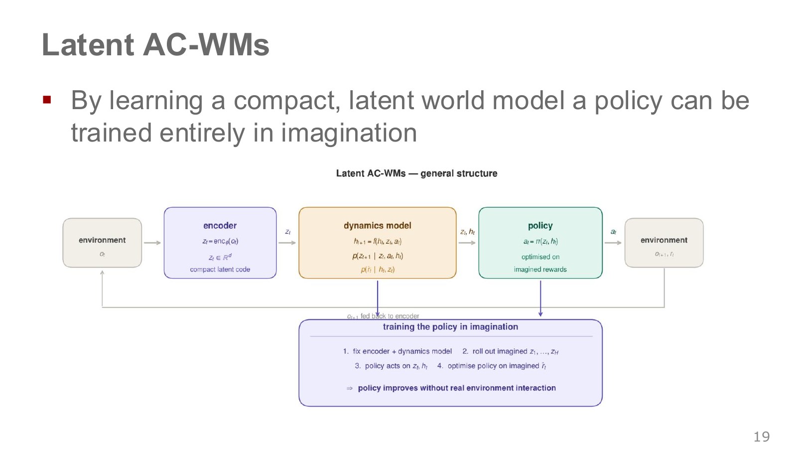
The encoder on the left maps observations to vectors. The dynamics model in the middle predicts vectors and rewards given actions. The policy selects another action and feeds it back into the dynamics model. The lower loop improves the policy through these predicted experiences. Distinguishing real environment data for model learning from model-generated data for policy learning reveals the figure’s two paths.
A latent code compresses an image into numbers useful for control. Representing cup and arm positions without every background pixel makes candidate comparison cheaper. But losing a small cup handle or a narrow pre-contact gap can harm grasping even when reconstruction looks plausible. Evaluate visual fidelity and actual control success separately.
#P021 · V sees, M remembers, and C chooses actions
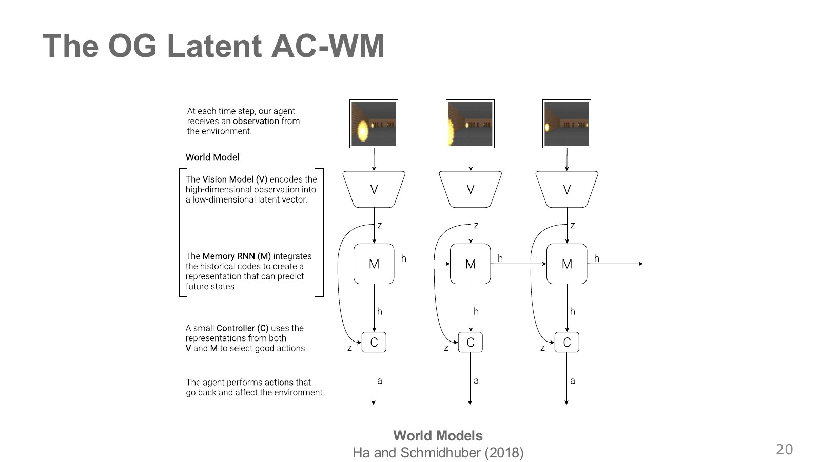
In Ha and Schmidhuber’s figure, V compresses the current frame, M remembers previous scenes and actions, and C selects actions from both current vision and memory. Remembering which way a road curved can guide steering even after the bend leaves view. Ha and Schmidhuber, World Models
#P022 · Reconstruction reveals compression's gains and losses
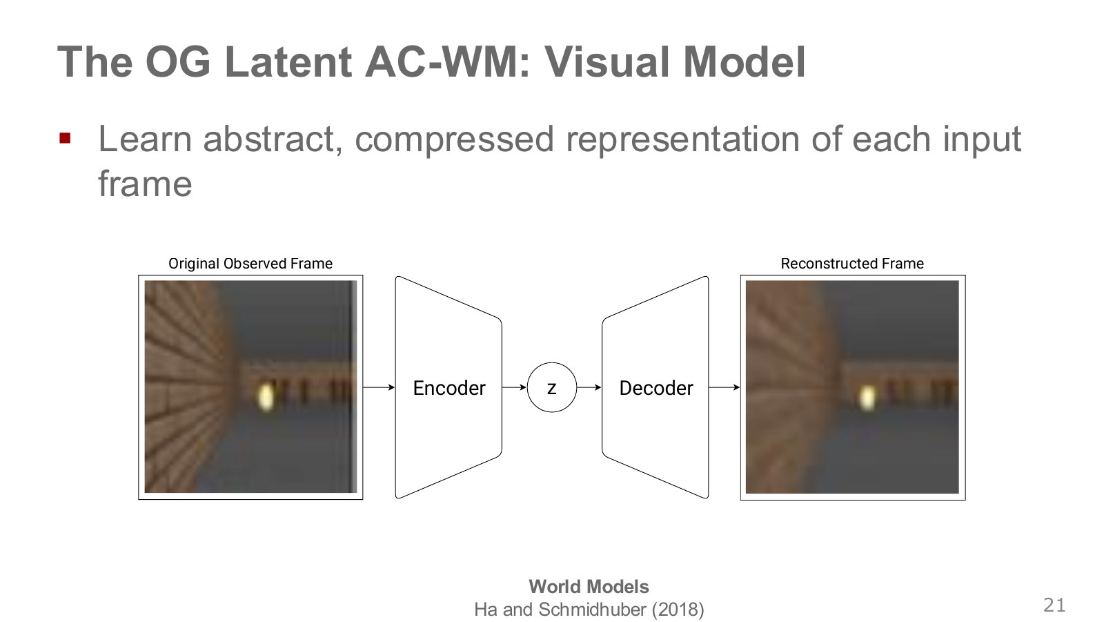
The game frame on the left is compressed by a VAE encoder and reconstructed by its decoder on the right. Corridors and bright objects remain while surface textures blur. This may suffice for avoiding walls but fail if a small wall sign marks the destination. Reconstruction quality and preservation of task-relevant information need separate evaluation.
#P023 · Do not collapse alternative futures into one mean
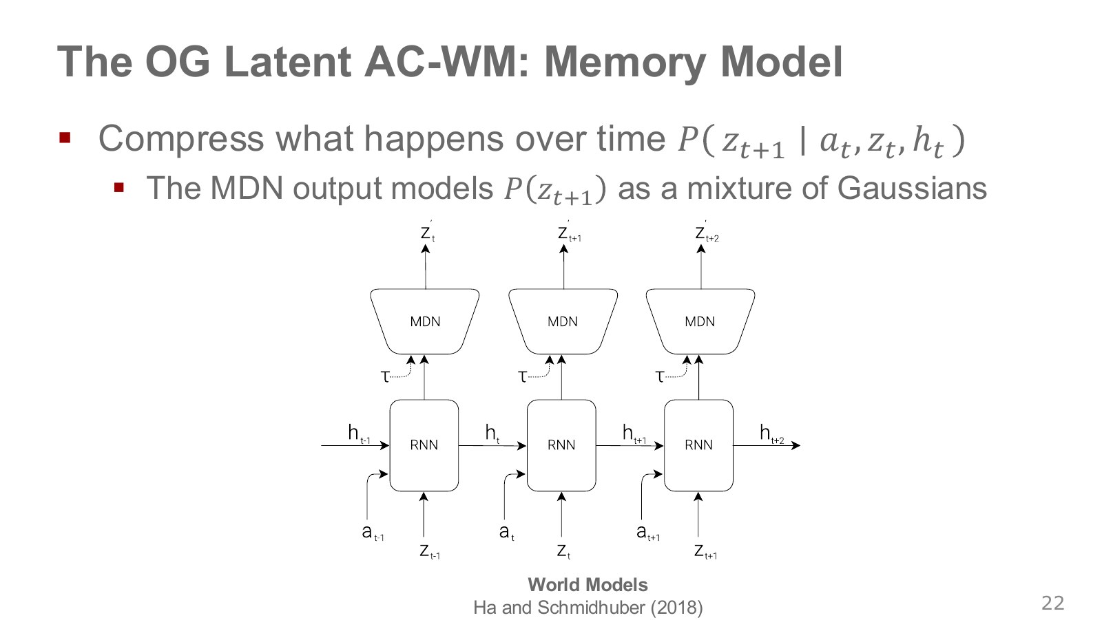
The RNN carries memory forward. The mixture density network (MDN) above it represents the next latent-value distribution with multiple Gaussian components. If a ball can bounce to either side of an obstacle, a mean-only prediction may send it through the middle. Retaining probability near both outcomes lets those futures be evaluated separately.
Explore the symbols and calculation A mixture distribution representing alternative futures
Read the equation in words
Place multiple bell-shaped distributions near possible futures and combine them with different component weights.
Understand each symbol
- Latent vector of the next scene
- Component mixture weight
- Component center
- Within-component spread and direction
Follow the calculation
- Feed the current scene, action, and memory into the network to obtain component centers, spreads, and weights.
- To sample one prediction, first select a component according to its weight, then sample a value within that component.
Check with a small example
If left and right bounces have weights 0.7 and 0.3, about 70% of repeated component selections come from the left component.
An illustrative example for understanding the equation.
#P024 · CMA-ES tests candidate policy weights
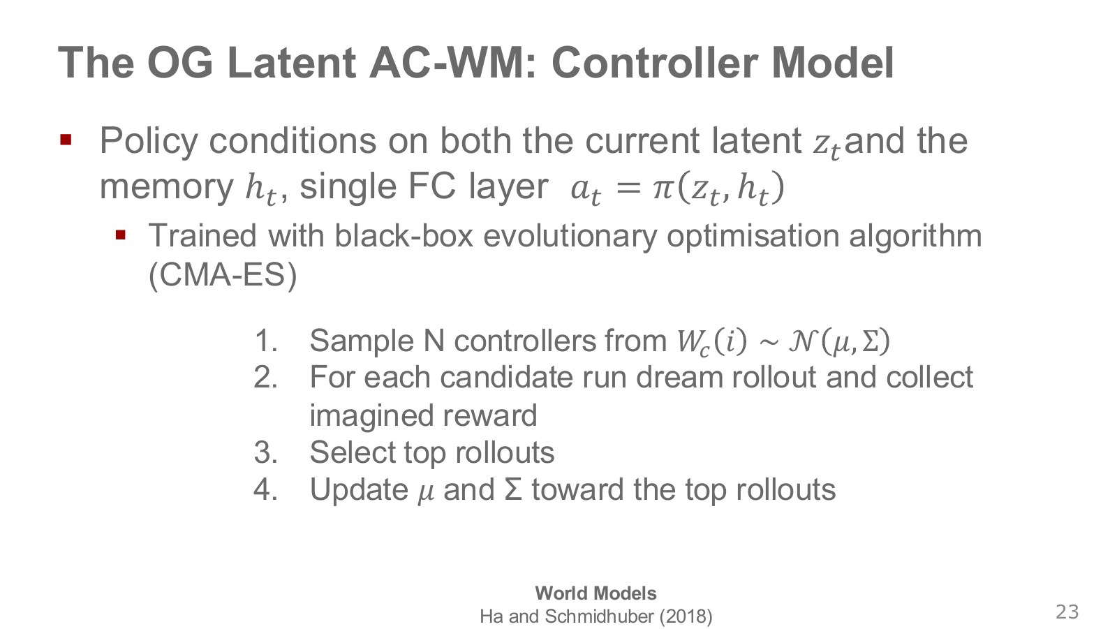
CMA-ES samples controller weights, runs an episode with each controller, and adjusts the sampling mean and covariance to favor higher-reward candidates in the next generation. Like CEM on P018, it evaluates candidates, but optimizes reusable controller weights rather than an immediate command sequence. The original paper uses the original environment or a learned dream environment depending on the task.
The controller C can remain small because V and M already represent scenes and temporal changes. C has less need, for example, to estimate speed anew from every frame. The original paper tests candidate C weights with the evolutionary strategy CMA-ES, compares cumulative dream-environment scores, and improves the next candidate population. This optimization is separate from training M to predict next latent states. Ha and Schmidhuber, World Models
#P025 · Why do corners become harder without memory?
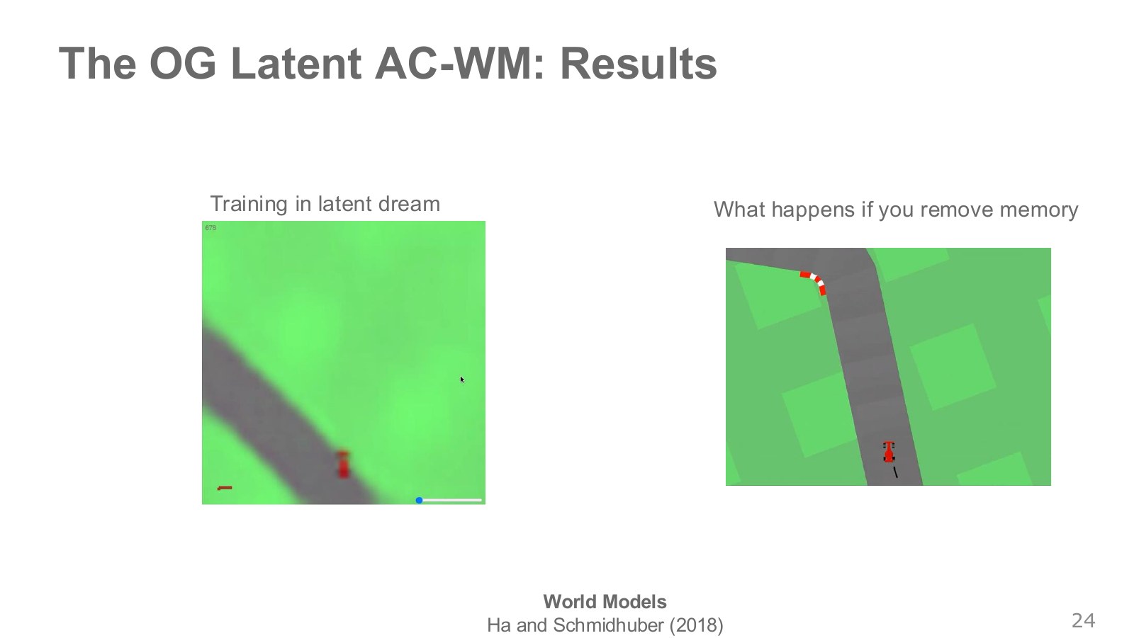
The right figure examines memory’s role. Even with only part of the road visible, earlier frames showing the bend provide steering evidence. Removing a module and measuring performance change on the same task is an ablation study. These results need not generalize unchanged to other robots whose observations already contain sufficient memory-related information.
#P026 · Test a dream-trained policy in the original environment
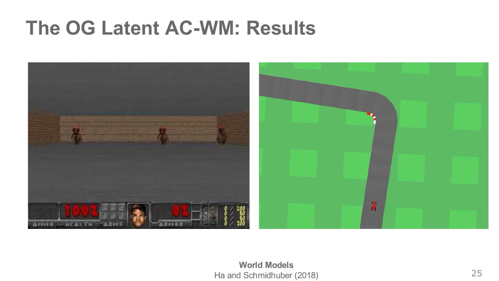
The left shows a Doom-style environment and the right CarRacing. In the original Doom experiment, a controller was trained inside the learned environment and then evaluated in the original game. Exploiting flaws missed by the dream model can reduce performance in the original game. The authors varied dream-environment sampling temperature to avoid excessively confident predictions.
#P027 · One step's error becomes the next step's input
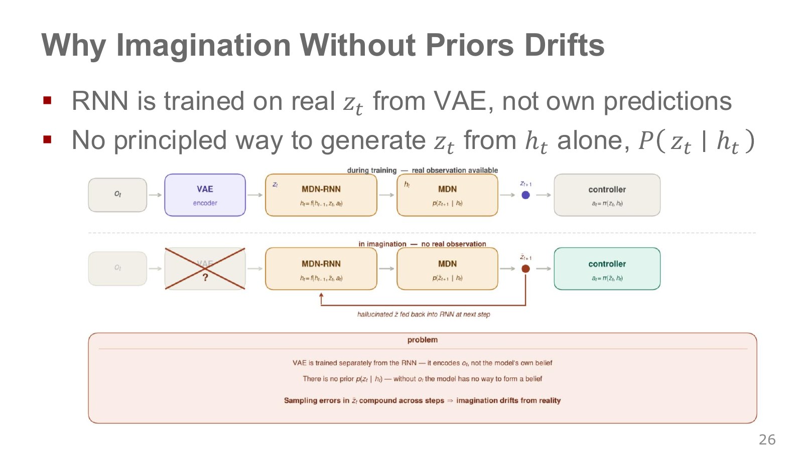
The upper path receives encoded actual frames, while the lower path feeds back model-generated latent values. If a predicted cup drifts sideways, the next prediction starts from that incorrect position. The earlier MDN-RNN already has a transition distribution for sampling futures. The RSSM introduced next separately learns an estimate before observation and an observation-informed estimate for the same time step.
#PlaNet and Dreamer
#P028 · RSSM learns predictions alongside observation-informed estimates
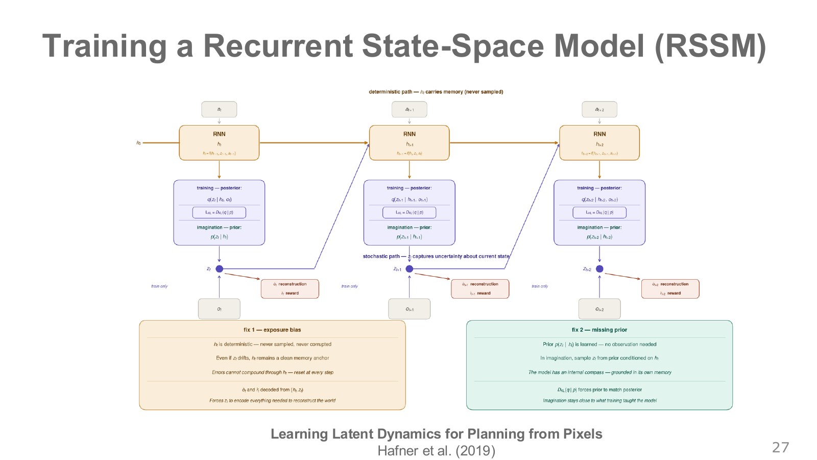
The orange RNN path carries memory from prior latent states and actions. The green prior estimates before seeing the new image; the purple posterior estimates after seeing it. Remembering that the hand reached forward does not reveal whether grasping succeeded. A photograph showing the lifted cup updates the estimate. Training brings the distributions closer while also explaining observations and rewards. Hafner et al., PlaNet
Explore the symbols and calculation RSSM prediction and observation correction
Read the equation in words
First update memory from the previous state and action. Use it to predict the future, then correct the latent-state estimate when an actual observation arrives.
Understand each symbol
- Recurrently passed memory
- Stochastically represented latent state
- New sensor observation
- The prior and posterior, respectively
Follow the calculation
- Predict grasp success from the preceding frame and gripper-closing command.
- If the next frame still shows the cup on the table, the observation-informed estimate incorporates that information.
Check with a small example
For example, a prior predicting grasp success at 0.7 may be corrected downward when a clear photograph shows an empty hand.
An illustrative example for understanding the equation.
Read the prior and posterior through cup grasping. A history showing the arm rising does not establish that it lifted the cup. The history-only prediction is the prior. If a new photograph shows the cup still on the table, the observation-informed posterior shifts toward a failed grasp. Training fits reconstructions and rewards while reducing KL between these distributions, teaching plausible history-based state samples even when future images are unavailable during imagination.
The RSSM’s deterministic memory path carries history continuously, while stochastic latent variables represent alternative current situations consistent with it. A deterministic RNN path does not eliminate all noise: errors in predicted and sampled inputs still affect it.
#P029 · Feedback inside imagination versus feedback from the real environment
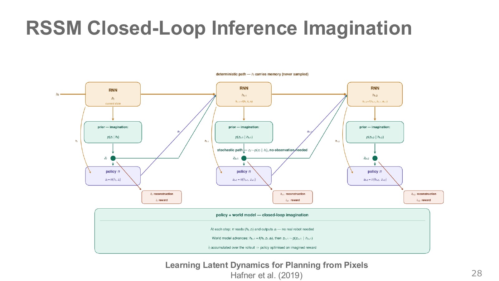
In the lower loop, the policy reads a predicted state to select an action and the model predicts again from that action. This loop closes within imagination. Without new real observations, future latents are sampled from the prior. During real execution, sensors correct the state estimate. Distinguishing these loops explains why RSSMs still accumulate error over long imagined trajectories.
Although a fixed function updates RSSM hidden state, its previous latent input already contains sampling and prediction errors. Training the prior against an actual-observation-informed posterior reduces the imagination–observation gap. Long imagined paths still need checking against real observations.
#P030 · Dreamer moves repeated planning computation into training
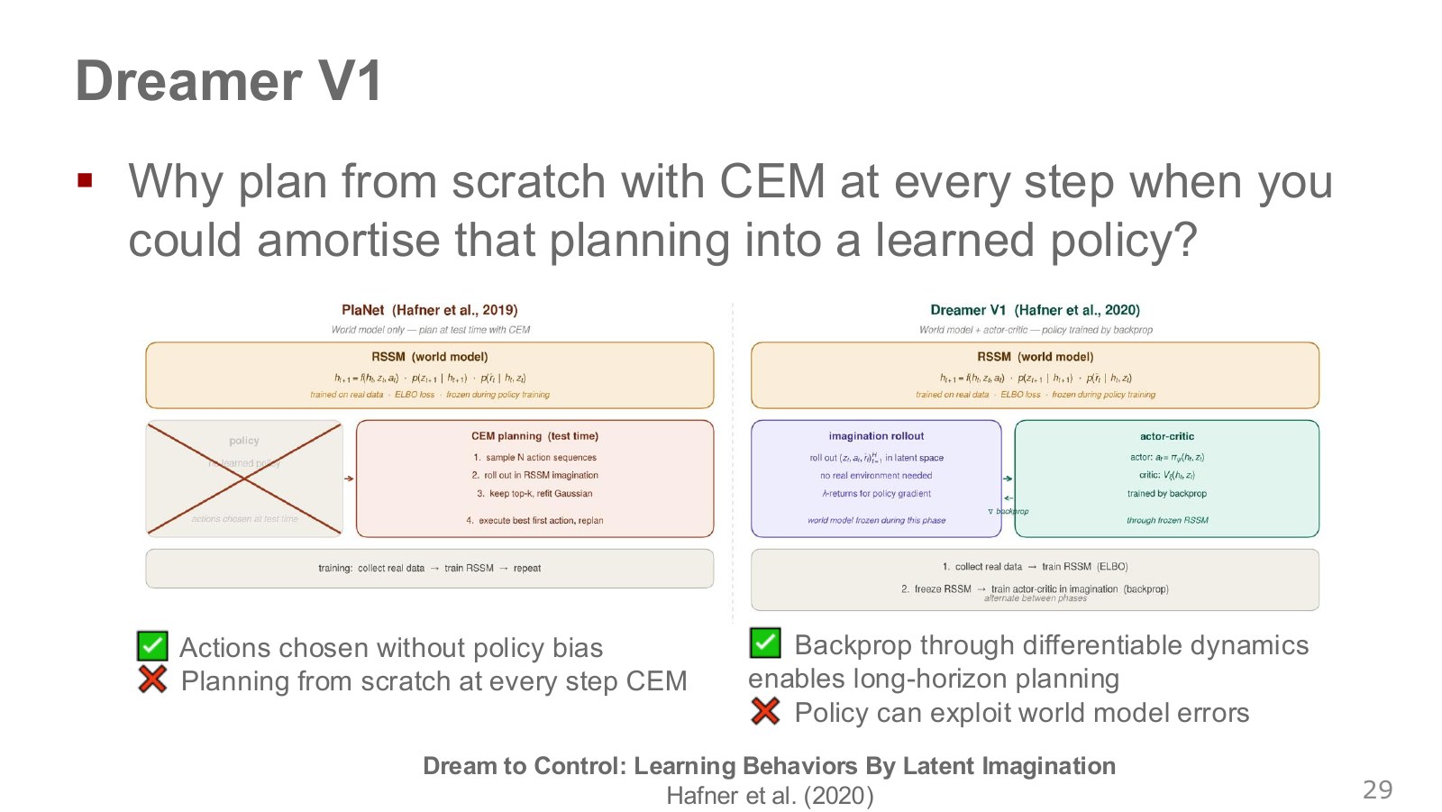
PlaNet on the left searches latent-space action sequences with CEM at every new observation. Dreamer on the right trains an actor to select actions and a critic to evaluate future rewards from imagined trajectories. Calling the actor at execution reduces repeated large candidate searches. But the actor may learn actions overvalued by the model, making real-environment validation important. Hafner et al., Dream to Control
Explore the symbols and calculation Discounted rewards along an imagined trajectory
Read the equation in words
Weight model-predicted rewards less heavily farther into the future and sum them. This shows the basic calculation over a finite imagination horizon.
Understand each symbol
- Model-predicted reward
- Discount factor
- Imagination horizon
- Sum of predicted discounted rewards
Follow the calculation
- Advance the world model repeatedly using actor-selected actions and obtain rewards at each step.
- This sum illustrates comparison of candidate policies. Actual Dreamer also uses value estimates beyond the horizon.
Check with a small example
With discount factor 0.9, current reward 1, and next reward 2, the sum is 1+0.9×2=2.8.
An illustrative example for understanding the equation.
Dreamer first updates a world model to explain images and rewards from real trajectories. It then starts imagined trajectories from latent states of real experience. Model weights are held fixed during this policy update, while the critic estimates cumulative future rewards. Across overall training, fresh real experience continues updating the world model. This differs from permanently freezing a model after its initial creation. Dreamer V1
#P031 · DayDreamer applies the approach to real robots with sensors and motors
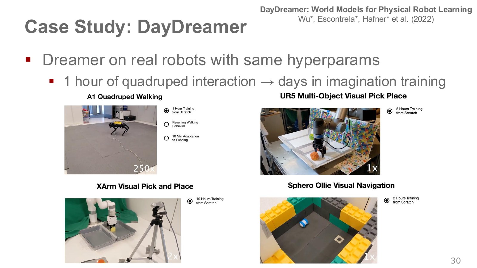
The four photographs show A1 quadruped locomotion, UR5 object transfer, XArm grasping, and Sphero navigation. Learning to stand and walk from about an hour of real quadruped experience and the arm-manipulation experiments are separate tasks. Motor control and learning must run concurrently on physical robots, so the authors execute collection and training asynchronously. Wu et al., DayDreamer
#P032 · A cinematic training-room analogy locates the computation
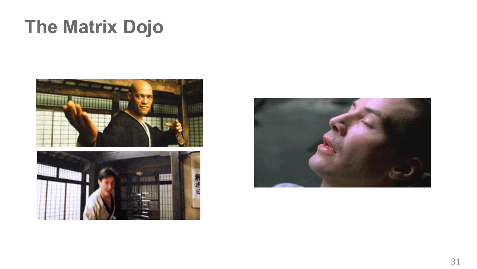
The person on the left practices in a virtual dojo while the person on the right remains in reality. In world-model imagination, GPUs rapidly replay transition patterns learned from past data. If the virtual floor is less slippery than reality, a gait learned only there may be unsafe. The analogy illustrates both moving practice elsewhere and checking the learned result in reality.
#P033 · What changes from World Models to Dreamer V4?
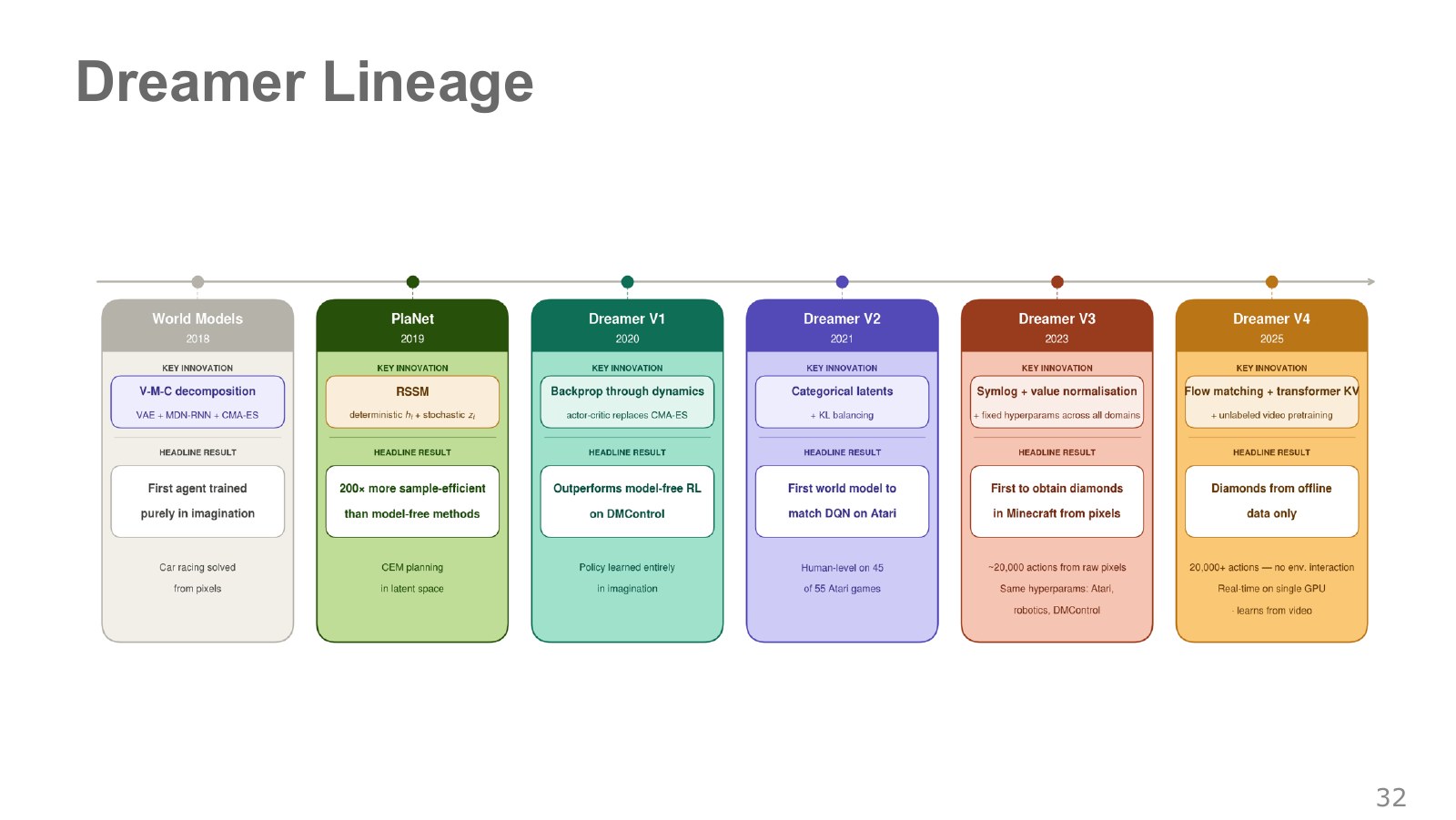
Reading left to right gives separate vision/memory/control modules in V/M/C, latent planning with PlaNet’s RSSM, imagined policy learning in Dreamer V1, categorical latents in V2, stabilization across reward scales in V3, and scaling to larger video datasets in V4. This is not a same-condition benchmark comparing every successor against every predecessor; read each card’s achievements with its paper’s tasks. Dreamer V2 · Dreamer V3
| Study | Main change | Conditions to check when reading results |
|---|---|---|
| World Models | Separate VAE, MDN-RNN, and controller | Which games transfer from dream training to the original environment |
| PlaNet | RSSM combining deterministic memory and stochastic states; latent-space CEM | Candidate-planning cost at each observation |
| Dreamer V1 | Train actor and critic through imagination | Roles of real and imagined data |
| Dreamer V2 | Categorical latents and improved KL learning | Changes in representation and training stability |
| Dreamer V3 | Stabilization across reward and observation scales | Evaluations across domains including Minecraft |
| Dreamer V4 | Scalable video models and offline imagined learning | Action labels in training data and use of online experience |
Obtaining a diamond in Minecraft is a long task requiring wood, tools, and mining in sequence. As the lecture moves from V3 to V4, it emphasizes which data teach this long-horizon behavior. Distinguishing action-free video pretraining, action-labeled adaptation, and imagined policy training reveals where general video is used. Dreamer V3 · Dreamer V4
#P034 · Dreamer V4 separates video pretraining from action learning
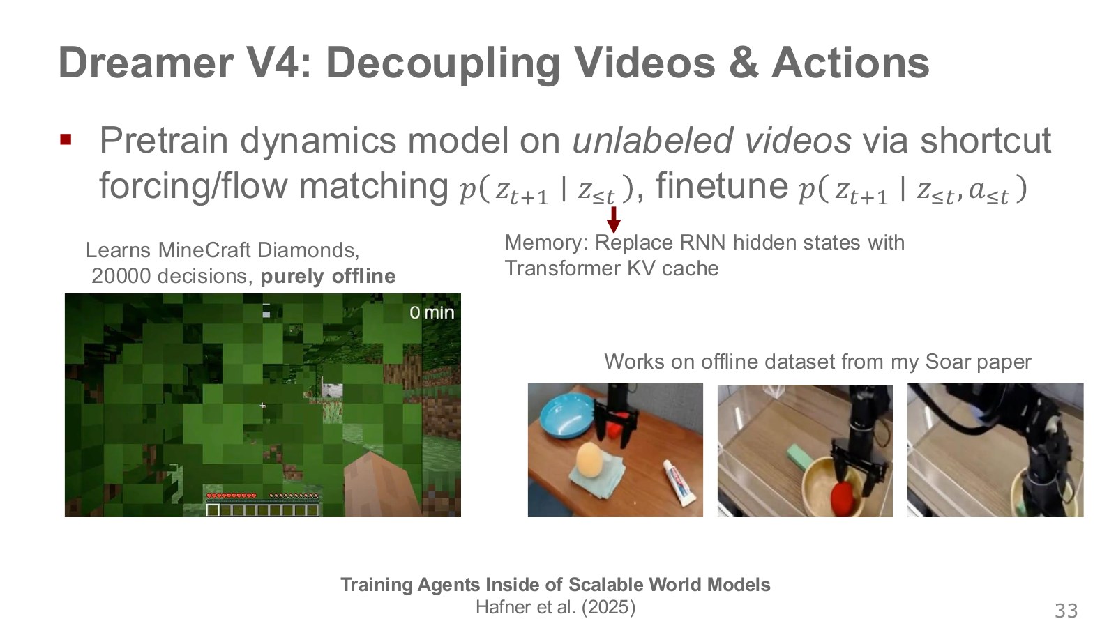
The Minecraft scene on the left illustrates an agent learned from offline data. Video without action records can teach temporal scene changes. Subsequent action-labeled data are needed to identify which commands cause which changes. V4’s Minecraft result belongs to its specified data, action space, and evaluation. The robot image on the right is a separate data-application example discussed in the lecture. Hafner et al., Dreamer V4
Explore the symbols and calculation Pretrain without action labels, then add action conditioning
Read the equation in words
First predict continuations of observed video; later, also accept recorded commands to predict their effects.
Understand each symbol
- Video representations through the current time
- Action history through the current time
- Model parameters in the two training stages
Follow the calculation
- For video without action labels, predict the next frame from preceding frames.
- Adapting on data with recorded robot commands allows testing different commands from the same scene.
Check with a small example
Video of a person moving a cup provides motion cues. Command-labeled robot data connect those cues to the meaning of moving a robot hand 2 cm right.
An illustrative example for understanding the equation.
#Large-scale video and robot actions
Another V4 change highlighted in the lecture replaces fixed-size recurrent memory with Transformer context and a KV cache. A KV cache stores keys and values of previously read tokens for reuse in later predictions, so retained information depends on context length and storage cost. Flow matching learns changes in video latents, while action-labeled data connect them to specific commands. Keep action-free pretraining, action conditioning, and imagined policy improvement separate rather than treating them as one training stage. Dreamer V4
The Dreamer V4 paper presents a Minecraft diamond task requiring more than 20,000 mouse and keyboard actions from pixel inputs. Intermediate resources and tools must be obtained in sequence over this long task. This length differs from the internal number of flow-integration steps generating one video. Original Dreamer V4 paper
#P035 · Extending game-specific latent representations through Internet video
A game limits the objects and camera movements frequently encountered. Internet video offers more varied objects and motion, but also varied viewpoints, backgrounds, and purposes. This motivates large video models. Useful robot representations must connect Internet-video patterns to robot viewpoints and manipulation data.
#P036 · Why can ten seconds of video contain 51,200 tokens?
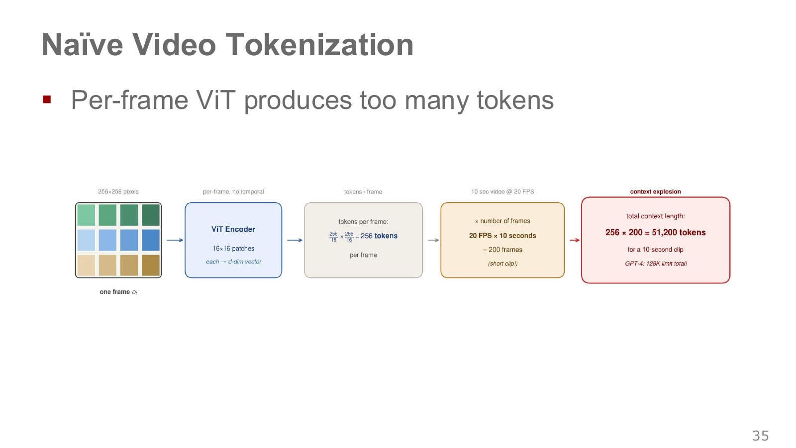
Each grid cell is a patch. A 256×256 image divided into 16×16-pixel patches has sixteen patches along each axis. At twenty frames per second for ten seconds, those 256 patches repeat across 200 frames. Standard dense attention compares all token pairs, so doubling tokens roughly quadruples comparison pairs.
Stanford CS231n’s ViT explanation projects each patch into a vector for Transformer input. Repeating this per video frame multiplies patches per image by frame count, as below. Justin Johnson, CS231n, 1:04:44 · Lecture slides
Explore the symbols and calculation Multiply patches per frame by frame count
Read the equation in words
Multiply patches across width and height, then by frame count to obtain the video's total token count.
Understand each symbol
- Total token count
- Pixels along one frame edge
- Pixels along one patch edge
- Frames per second multiplied by video duration
Follow the calculation
- Dividing a frame into sixteen patches horizontally and sixteen vertically gives 256 patches.
- Ten seconds at twenty frames per second gives 200 frames, so the result equals adding 256 two hundred times.
Check with a small example
Five seconds at the same resolution and frame rate gives 25,600 tokens. Frame grouping or additional tokens changes actual input length.
An illustrative example for understanding the equation.
#P037 · Compress space and time while allocating tokens to important regions
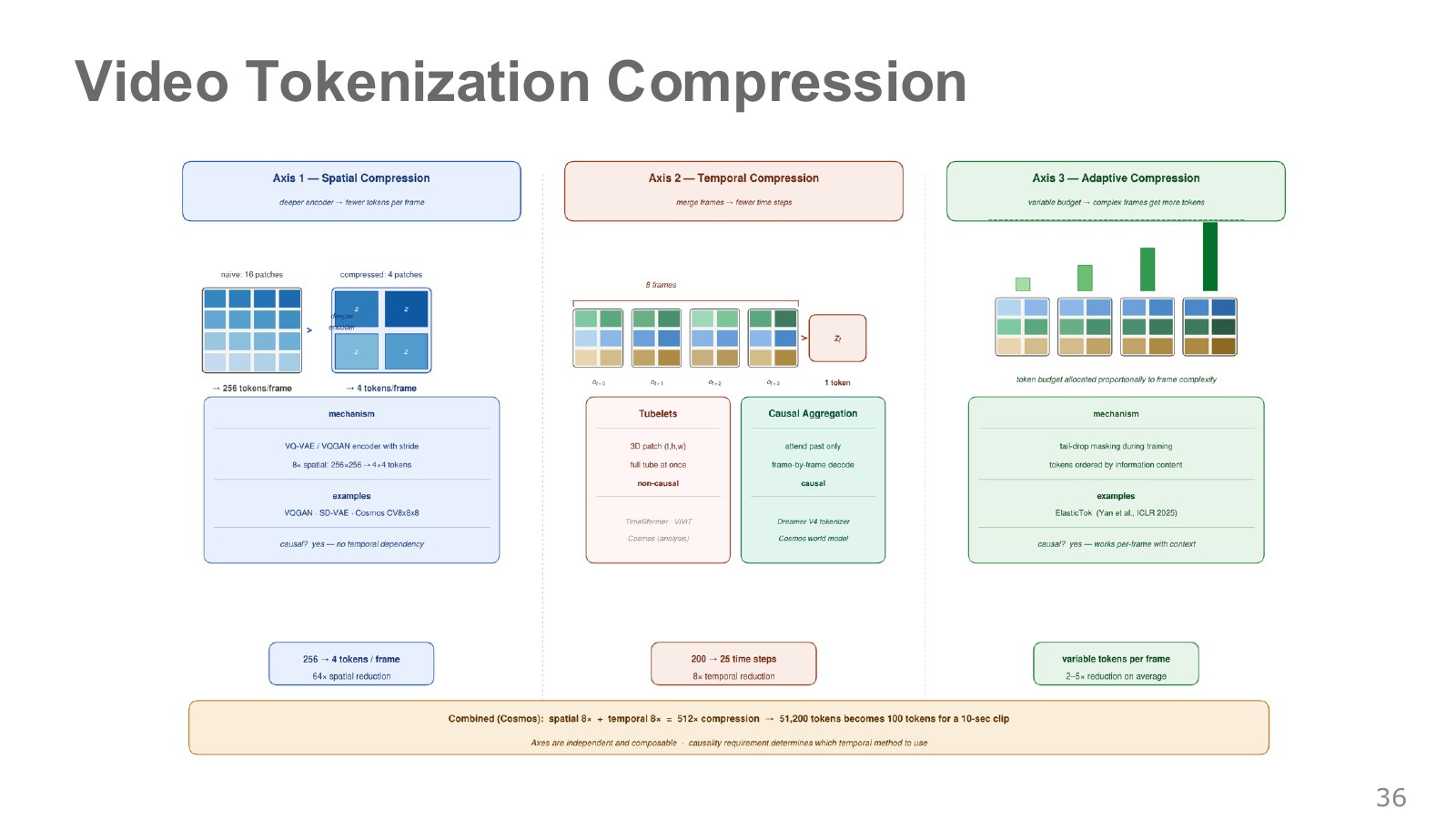
The first column groups neighboring locations spatially, the second groups change across frames temporally, and the third allocates tokens adaptively by scene. A stationary wall may tolerate strong compression, but coarsening a finger’s first contact with a cup handle can erase contact timing. The slide’s compression numbers illustrate principles.
Using future frames for temporal compression is convenient for recorded video, but real-time control cannot use frames that have not arrived. Commands must be based on tokens formed from frames available so far. Static backgrounds and rapidly changing contact scenes also need not receive equal token budgets.
Three axes clarify compression. Spatial compression groups neighboring pixels within a frame. Temporal compression groups repeated information across frames. Adaptive compression aims to allocate fewer tokens to stationary walls and more to changing hands and objects in contact. These choices can be combined, but token-count calculations must separately account for both spatial axes and time.
The lecture’s large compression factors are conceptual approximations. Actual token counts require input resolution, temporal sampling, latent-grid sizes, and token definitions. A label of “8× compression” alone does not support comparing context lengths across models.
Consider a hypothetical eightfold reduction along width, height, and time. A 256×256-pixel, 200-frame input becomes a 32×32×25 latent grid with 25,600 positions. That is 1/512 of the original 13,107,200 pixel positions, but only half the previous page’s 51,200 patch tokens. Applying pixel-based compression again to an already patched token count is incorrect. This educational calculation treats each latent position as one token and does not claim an actual Cosmos configuration’s output length. The transcript’s “about 100” cannot be derived from these factors alone without input resolution, latent-grid, and further patching details.
#P038 · First ask whether actions are model inputs or outputs
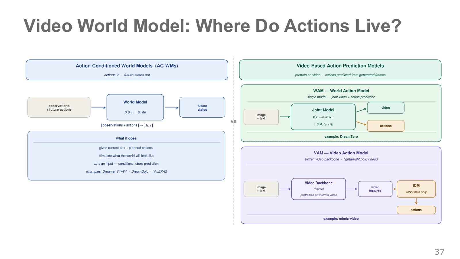
The action-conditioned model on the left answers “What happens if I push right by 2 cm?” with a future state. DreamZero at upper right jointly outputs future video and actions, while mimic-video below decodes commands from intermediate video-model features. All use video, but differ in whether candidate actions must be supplied and where executable commands originate.
| Category | Model input | Output | Use in planning |
|---|---|---|---|
| Action-conditioned world model | Current observation/memory and candidate actions | Next-state and reward distributions | Vary actions and compare outcomes |
| WAM: DreamZero example | Observations, instructions, etc. | Future video and corresponding actions | Execute jointly generated action chunks |
| VAM: mimic-video example | Video features conditioned on observations/instructions | Commands from an action decoder | Translate visual plans into control values |
WAM means World Action Model and VAM Video Action Model. Later in the lecture, both approaches are sometimes grouped broadly together. Following whether actions enter or leave the model, and whether a separate decoder is used, is more informative than names alone.
#P039 · Why use expensive video computation in pretraining?
Video pretraining can expose a model to many scenes of objects rolling or following a hand. Execution may reuse only the learned features. Separate video-training cost from the latency of issuing one motor command.
#P040 · Static-image meaning differs from the rules of motion
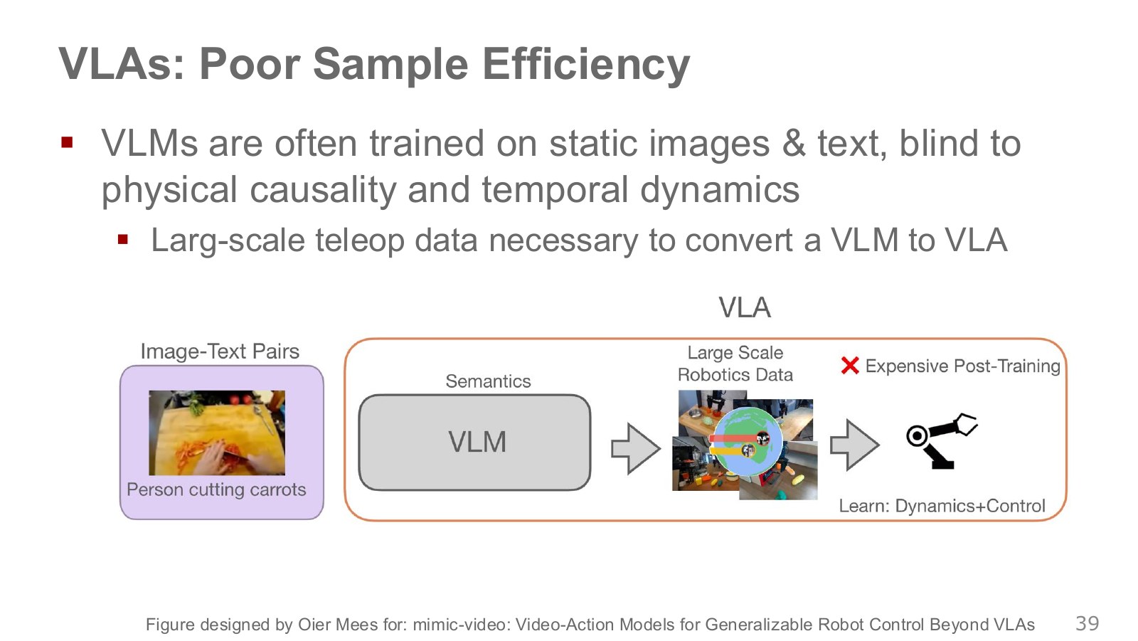
An image and caption can identify a carrot and knife. Consecutive frames more directly reveal pressing order, direction, and where cut pieces move. The lecture’s VLA comparison concerns transferring VLMs pretrained mainly on static images and text to robots. If a model already includes video or robot experience, first examine its actual training data.
#P041 · Learn motion from video and commands from robot data
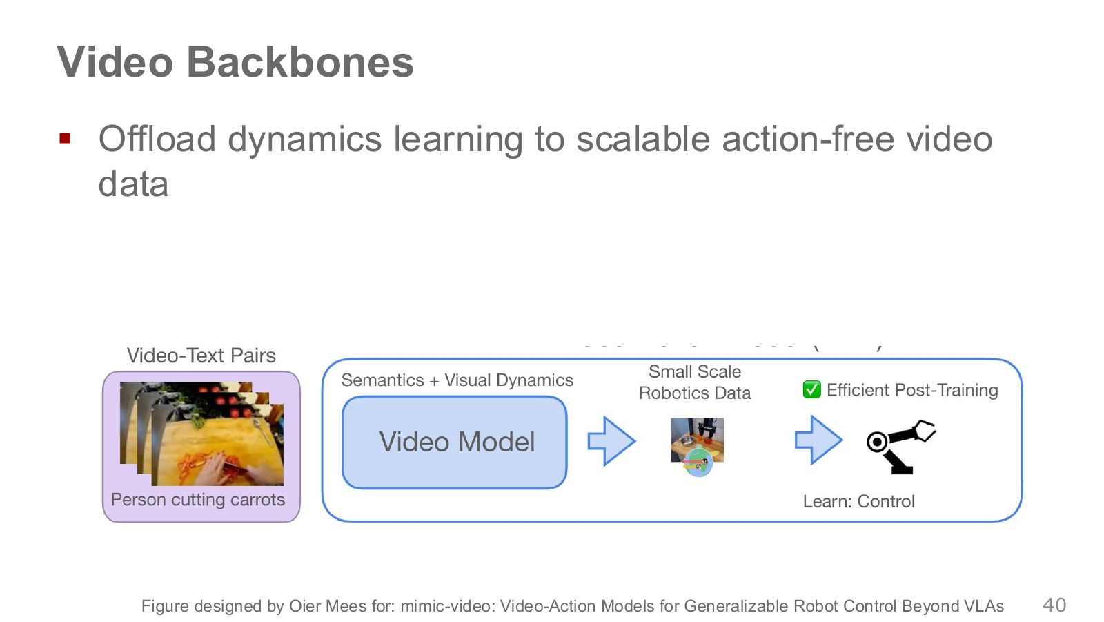
Video–text inputs usually do not include robot joint angles or motor torques. They can still teach temporal cues from objects following hands. Robot-specific actions require data pairing camera observations with commands. Human hand motions therefore cannot simply be copied into robot motor commands.
#P042 · mimic-video attaches an action decoder to video features
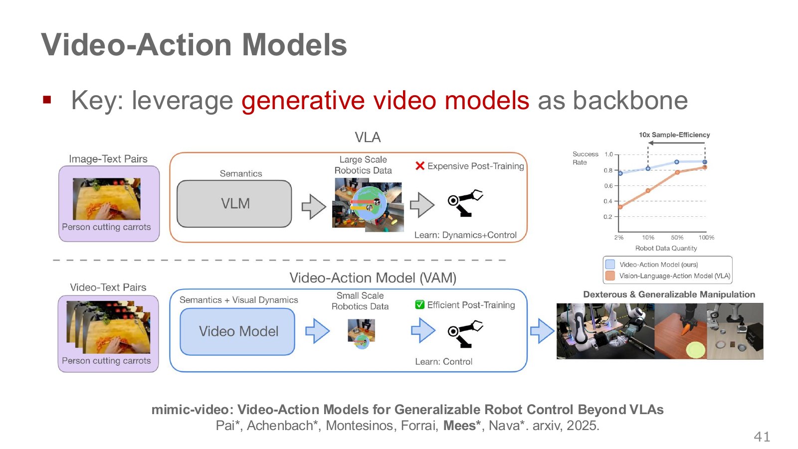
The upper path adapts a VLM to robot actions; the lower uses a generative video backbone. In mimic-video, an action decoder produces robot commands corresponding to anticipated visual changes. Inferring actions from resulting changes makes it an inverse dynamics model (IDM). Several joint motions can produce the same visual change, and training data influence which command is chosen. Pai et al., mimic-video
#P043 · What improves when the decoder receives expert video?
The graph separates predicted-video inputs from expert-video inputs. Expert video provides an experimental reference containing outcomes unavailable in advance during deployment. Higher success with this input indicates room to improve video prediction. Failures remaining with expert video also require examining action decoding and robot execution. Since the copied figure’s bars are not visible, the lecture explanation and paper supplement the comparison and interpretation. mimic-video
The paper’s oracle condition supplies latent representations extracted from actual future frames. Near-perfect success under that condition indicates substantial room to improve predictions in that comparison. mimic-video paper
#P044 · Use intermediate denoiser features rather than completed video
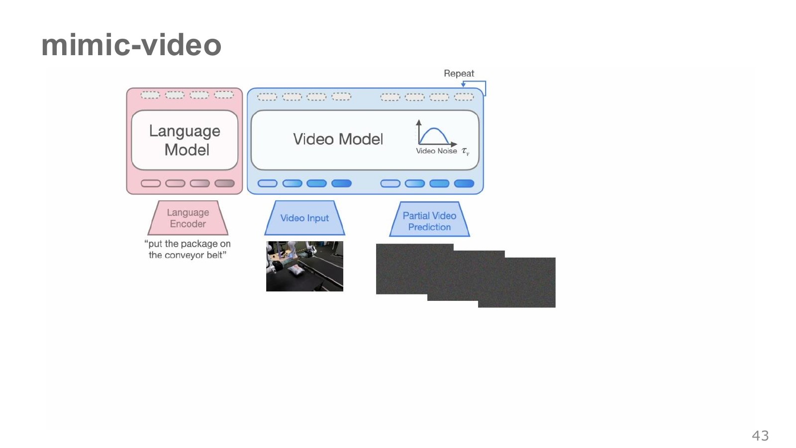
The pink language model handles instructions, while the blue video model handles current images and partially refined future representations. Even noisy intermediate features can contain object-motion and task-direction information. The decoder generates action chunks from them, reducing the need to render visually polished video in the normal control path.
Features from mimic-video’s Cosmos-Predict2 can be extracted before reconstructing final RGB frames. How far video denoising proceeds before feature extraction and how many refinement steps generate actions are controlled separately. mimic-video paper
Video and actions generated through flow matching each have their own refinement progress. Video features can indicate where to move an object before final frames are complete. mimic-video conditions action generation on these intermediate features. Adjusting video and action refinement separately allocates computation according to action-generation needs rather than visual polish. mimic-video paper
#P045 · Simulation benchmarks and real dual-arm manipulation test different questions
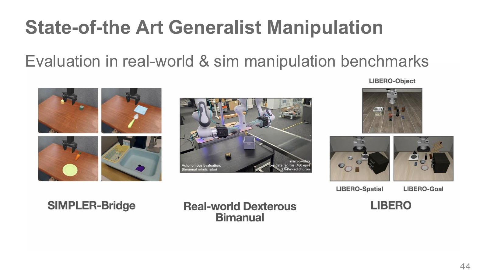
SIMPLER-Bridge compares manipulation in simulation. The middle shows real dual-arm manipulation; LIBERO’s Object, Spatial, and Goal splits separately test generalization across objects, layouts, and goals. Identical success percentages are comparable only with knowledge of what changed and how many trials were run.
#P046 · Data efficiency and training speed are different axes
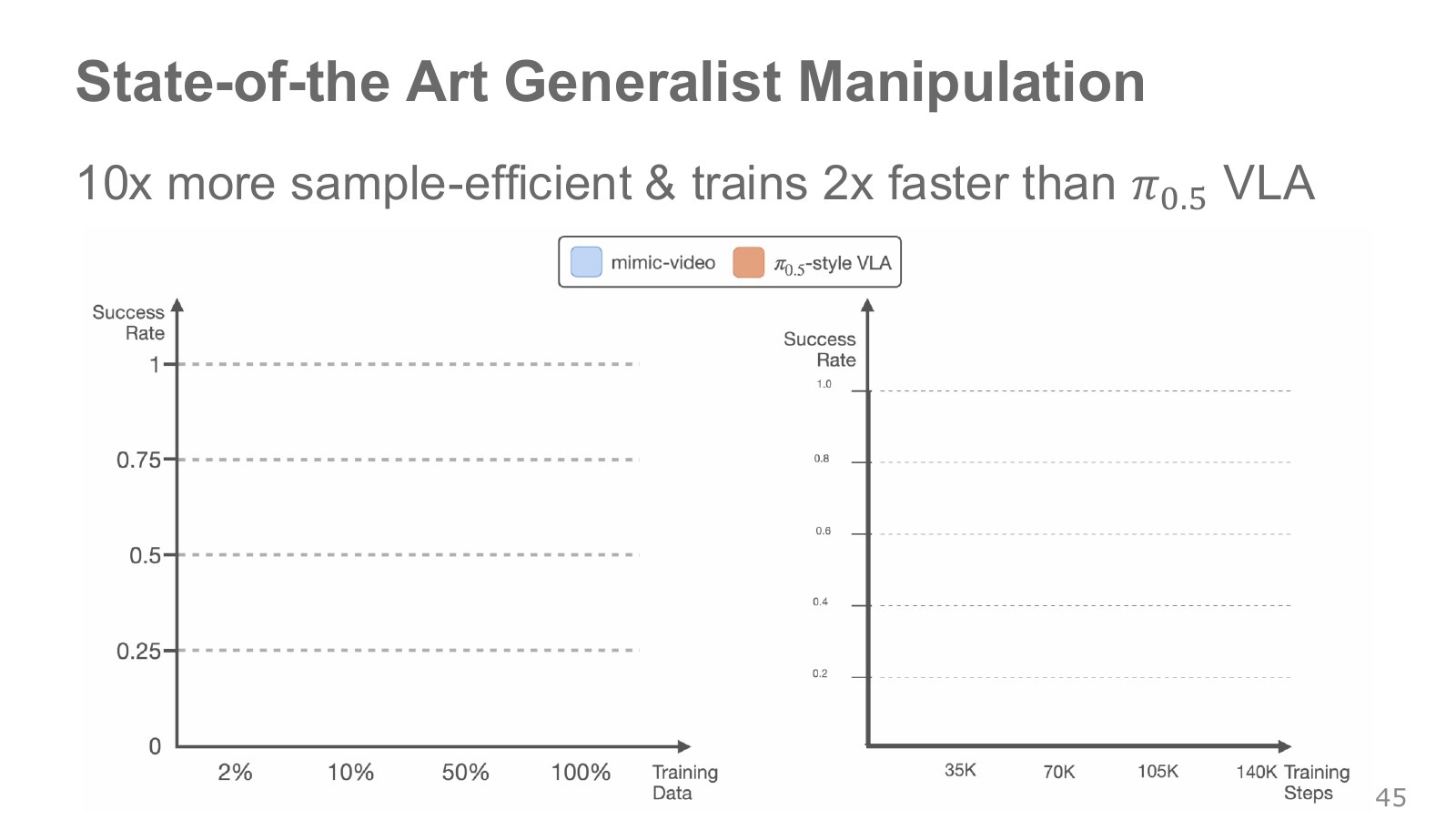
The left graph uses the fraction of robot data on its horizontal axis; the right uses training steps. The lecture’s approximately tenfold data efficiency and twofold faster learning refer to the authors’ comparisons of mimic-video with -family baselines. Fewer steps do not automatically mean less wall-clock time across different hardware or batch sizes. The copied axes and video explanation were read alongside the paper. mimic-video
#P047 · Actual execution on the left; model-generated video on the right
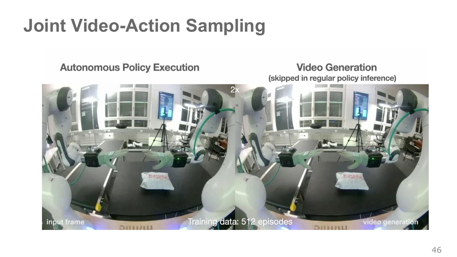
The scenes may look similar, but the left results from motor commands and the right from video generation. The slide states that video rendering is omitted during ordinary policy inference. The 512-episode label describes that demonstration’s setting. Task completion must be assessed through actual execution.
#P048 · DreamZero jointly predicts video and actions within one model
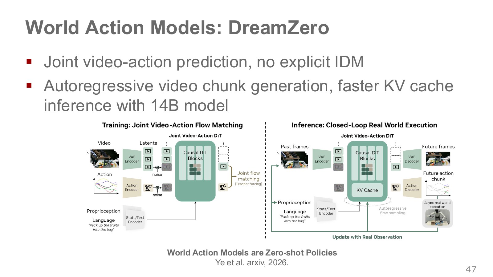
The left diagram adds noise to both video and actions and learns both outputs jointly. On the right, the robot executes an action chunk, receives actual frames, and generates the next chunk. A KV cache stores attention information from earlier frames to reduce recomputation. Ye et al., DreamZero
For example, the predicted gripper may hold the cup while the actual camera shows it still on the table. Updating the next chunk’s context with real frames creates an opportunity to approach again instead of extending the mistaken prediction.
DreamZero trains with actual past context and jointly predicts noise in future video and actions. Teacher forcing supplies correct preceding context during training. At inference, it executes a generated chunk and receives fresh observations before the next one. Replacing anticipated scenes with actual scenes reduces compounding error from continuing to assume an imagined cup was grasped.
A KV cache stores keys and values for processed context to reduce recalculation. Real-time operation of large models also requires system design such as cache management and fewer generation steps. Future-video quality alone does not determine actual control speed. DreamZero paper
The lecture emphasizes implementation choices enabling real control rates even with DreamZero’s 14-billion-parameter model. Parameter count alone does not guarantee the same speed on another GPU or robot. Examine chunk-generation latency, executed chunk length, and how frequently actual observations update the cache together.
#P049 · Read new-task and few-shot adaptation results under their evaluation conditions
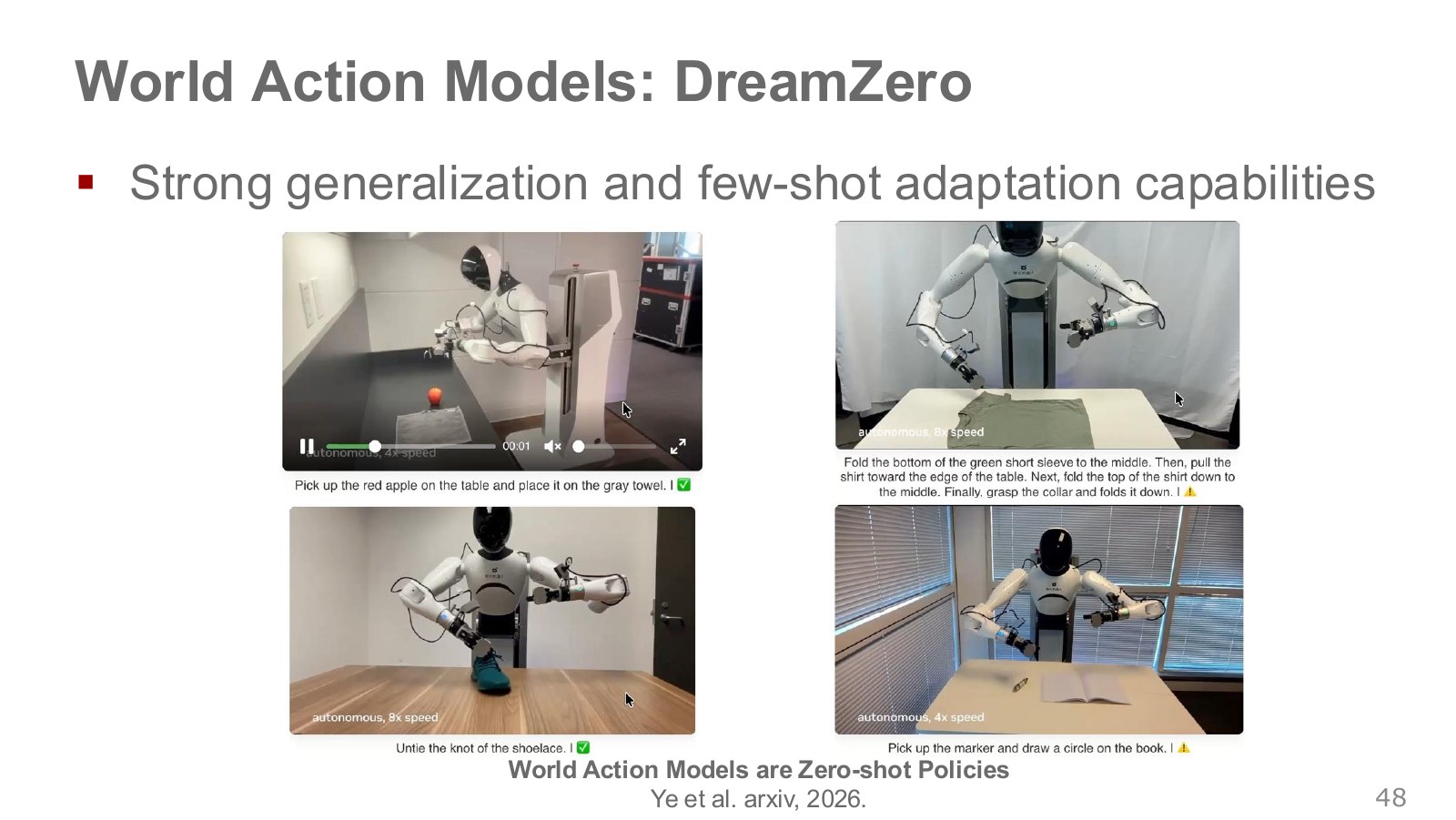
The photographs show moving apples, folding shirts, untying cords, and drawing circles. Familiar scenes can still require different action orders and contacts. Zero-shot means no additional training on that evaluation task; few-shot adaptation adjusts the model with limited additional data. Identify the setting even when interpreting demonstration photographs.
#P050 · When terminology differs between papers, compare inputs and outputs
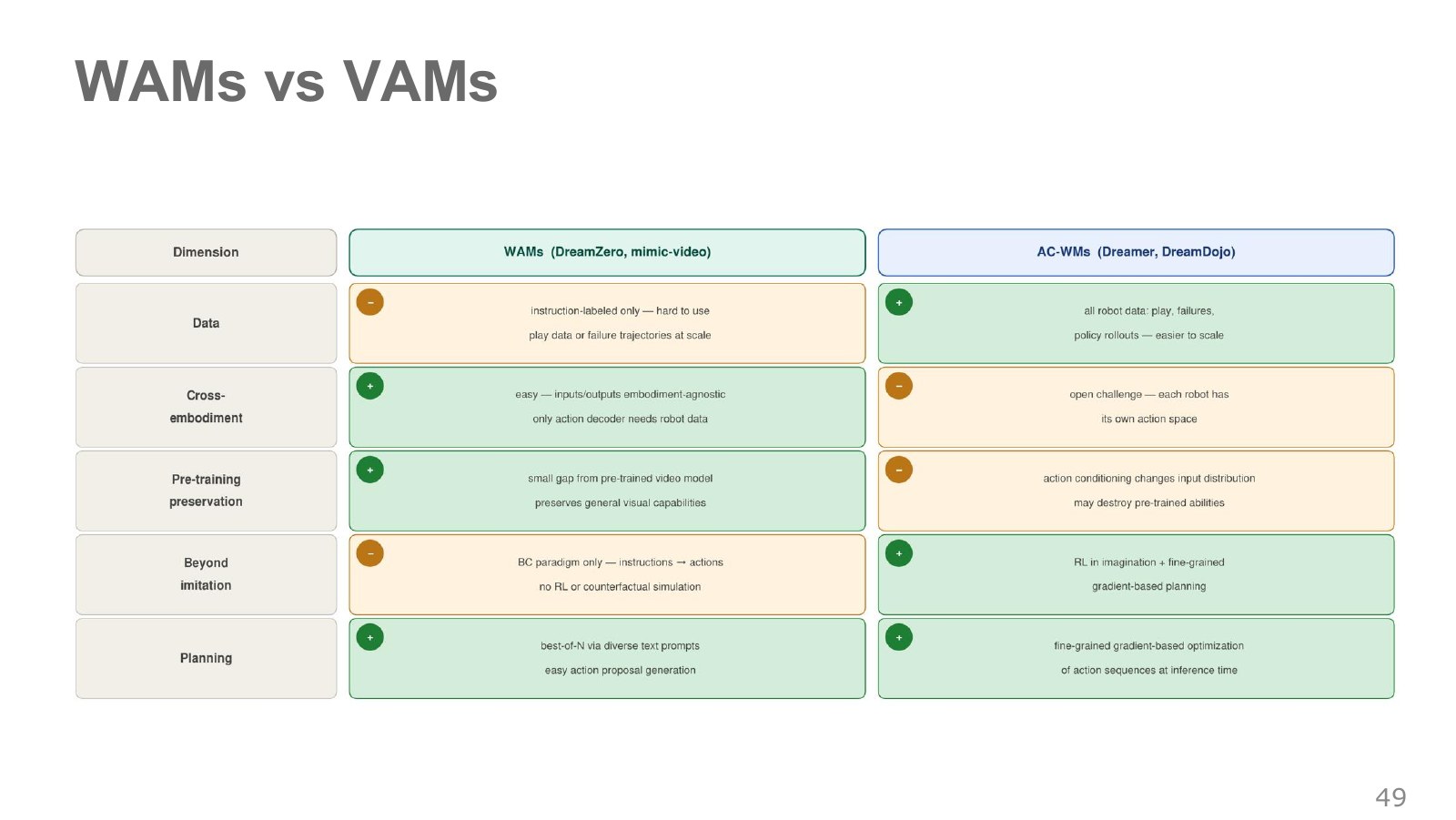
This table groups DreamZero and mimic-video together opposite Dreamer-style methods. P038 separated DreamZero as WAM and mimic-video as VAM. Despite changing categories, compare whether candidate commands can be varied to test outcomes, whether goals directly produce commands, and where robot data are required.
Action-conditioned models can learn what followed each action from failures, successes, and free play alike. Combined with learned reward models, they can support imagined reinforcement learning. Goal-conditioned action models may need annotations linking instructions to relevant segments. General video backbones can first learn motion from Internet video without robot commands, but connecting it to physical commands still requires robot data.
Cross-robot transfer can share video representations while adapting action decoders to equipment. Action-conditioned models likewise need ways to align different command semantics. Both evaluations must explain handling of robot-specific cameras and control units.
#Prediction without drawing pixels
#P051 · Must predicting contact also redraw the background?
Determining whether a cup is lifted does not require perfectly predicting wall textures. But losing the hand–cup gap during compression can ruin a grasp plan. This motivates JEPA, shifting prediction targets from pixels to task-relevant representations.
#P052 · JEPA predicts future-frame representations rather than future images
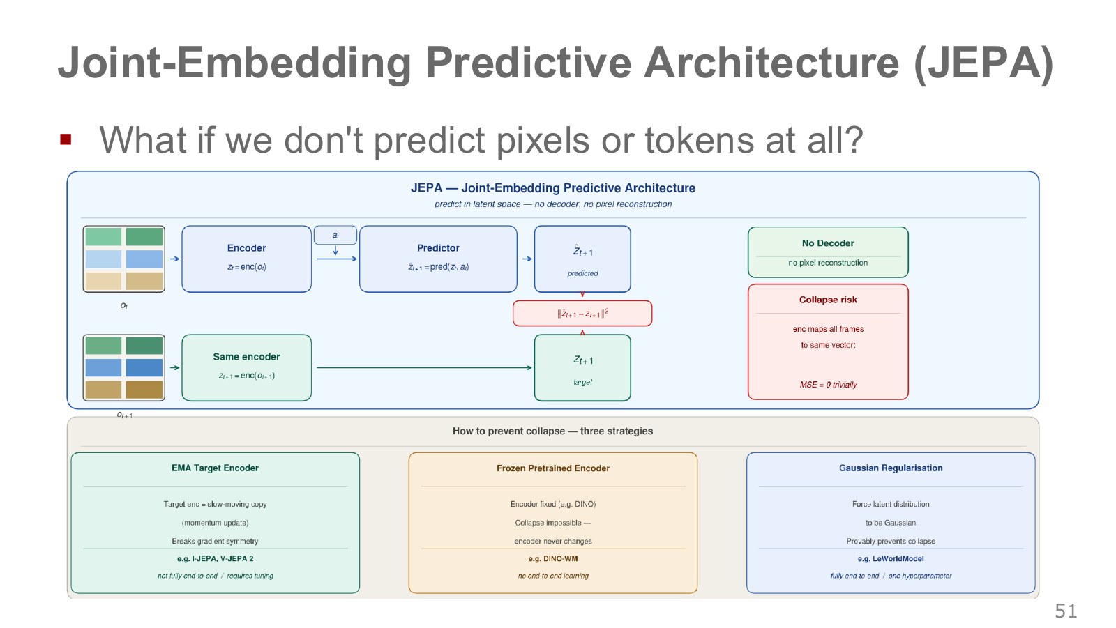
The upper predictor estimates the next representation from the current representation and action; the lower encoder converts the actual next frame into a vector during training. Comparing them avoids RGB reconstruction. If both paths map every scene to the same vector, error can be small but planning impossible: representation collapse. The three boxes illustrate slowly updated target encoders, pretrained frozen encoders, and distribution-spreading regularization. Their retained information and guarantees differ. V-JEPA 2 · DINO-WM · LeWorldModel
Explore the symbols and calculation Prediction error in future-scene embedding space
Read the equation in words
Compare the future vector predicted from current embeddings and an action with the actual next-scene vector, summing squared coordinate errors.
Understand each symbol
- Current-observation embedding
- Command supplied to the predictor
- Predicted vector
- Target encoded from the actual next frame
Follow the calculation
- Encode the current frame and supply it to the predictor together with the action.
- During training, also encode the actual next frame for comparison. Minimizing prediction error alone can collapse both representations to the same value.
Check with a small example
Prediction (1,2) and target (2,2) give summed squared error 1. Mapping every scene to (0,0) gives zero error but cannot distinguish objects.
An illustrative example for understanding the equation.
To picture collapse numerically, map both a lifted-cup image and an empty-table image to the same vector and have the predictor output only that vector. Prediction loss can be small without retaining grasp-success information. V-JEPA uses training designs including slowly changing target encoders. DINO-WM freezes pretrained DINO features and predicts future features. LeWorldModel suppresses constant solutions through Gaussian regularization spreading latent distributions. EMA alone does not automatically solve every representation-collapse problem.
In the learned representation space, action sequences can be selected to reduce distance between predicted future and goal-image features. To place a cup on a shelf, check whether predictions approach the goal, execute the first action, and update the state from the real camera. Final evaluation counts actual placement as well as representation error. V-JEPA 2 · DINO-WM · LeWorldModel
#P053 · Compare pixel and latent approaches through the same cup-transfer task
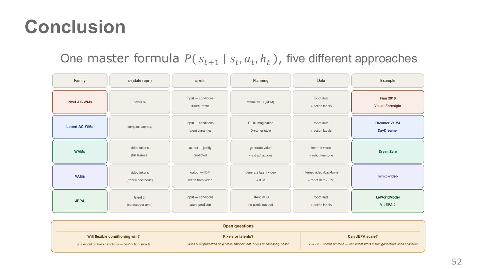
Pixel models predict where the cup moves in an image; Dreamer-style models evaluate multistep rewards or actions in compressed states. DreamZero jointly produces future video and commands, while mimic-video derives commands from video features. JEPA-based planning can compare predicted futures and goals as vectors. In every architecture, fresh observations after actual robot motion connect prediction with reality.
#Try the executable example
Suppose a virtual robot starts at position 0 with goal 1. Its model predicts that command 1 moves it by 1, but the example’s actual system moves only 0.8. Following the initial plan leaves it at 0.8. Observing the new position and commanding the remaining 0.2 brings it to 0.96; repeating once more reaches 0.992.
This example demonstrates the effect of observation-based replanning without changing the model. It uses only the Python standard library and includes neither a physical robot nor Dreamer training. Executable file and results