How does an instruction to move a hand toward a cup become motor motion? We will follow the path from coordinate frames through control, then connect it to a mathematical framework for evaluating and learning robot behavior.
Oier Mees · ETH Zurich 2026, Lecture 2 video · Official course · Original PDF
#P001 · From robot control to Markov decision processes
“Move your hand 1 cm toward the cup.” A short instruction hides several questions for a robot. In which coordinate frame is that centimeter measured? How far should each joint turn? How long should the motion take, and how should an overshoot be corrected? If the grasp misses, what should happen next?
In Chapter 01, a policy was a rule that receives information and chooses an action. Here we first examine how a chosen action becomes physical movement, then turn to Markov decision processes (MDPs) to evaluate the consequences of sequences of actions. The control in the first half and the learning in the second meet within one robot system.
#P003 · A common language for differently shaped robots
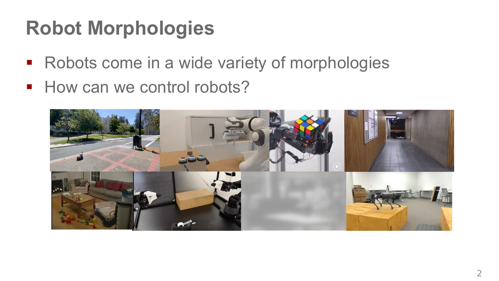
Drones move propellers, arms move joints, and mobile robots turn wheels. A robot’s morphology is more than its appearance. Joint connections, permitted directions of motion, and the arrangement of sensors and actuators determine which actions are possible.
The quadruped, Rubik’s-cube-solving hand and drone appear together because each must turn an abstract instruction into commands for its own body. The same instruction, “reach the target,” calls for adjusting motor thrust in a drone and joint commands in an arm.
Across hardware, the shared problem is turning what we want to do into commands the device can execute. Even “forward” means different things as a wheel speed, body velocity or target foot position. Whenever action appears in an equation, first ask which physical quantity is being commanded to which device.
The photographs show arms and hands manipulating objects, robots moving through corridors, and legged robots supporting their bodies. An arm controls contact between the tool and object; a mobile robot controls the relationship between its body and obstacles; a walking robot also controls foot contacts and balance. Even “move right” depends on what should move and what should stay fixed. Making that distinction first lets us define states and actions concretely. Video, 1:00–2:14.
A learning framework spanning these bodies cannot begin with memorizing the buttons on one particular arm. We need a common language for the relationships among goals, joint motion and actuator inputs. That is why rigid bodies, coordinate frames, joints and control come first here. Sharing a framework does not mean sending the same torque commands to every robot.
#P004 · Rigid-body motion: representing position and orientation together
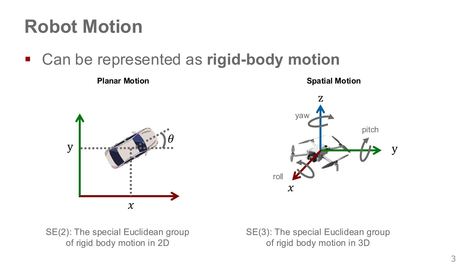
A rigid body is a model in which the distance between any two points in a body stays constant during motion. Approximating a metal link this way lets us describe its motion by the position and orientation of an attached coordinate frame, without tracking every surface point separately. It does not mean that a whole jointed robot is one rigid body.
Planar motion is usually described by two position coordinates and one orientation . The space of these poses is SE(2). Spatial motion requires position and three orientation degrees of freedom, represented using SE(3). A pose includes both position and orientation. Knowing a drone’s height alone does not tell us how it is tilted.
The rigid-body model uses the fact that points on one body move together to predict its next pose. Flexible cables and soft objects require deformation to be modeled separately. Six pose degrees of freedom also do not mean that a body can instantly move arbitrarily in all six directions. Actuators and contact constraints limit the motions actually available.
In the planar-car diagram, the straight arrows denote forward/backward and sideways position, while the curved arrow denotes heading. In the drone diagram, roll, pitch and yaw are rotations about the , and axes, respectively: tilting sideways, pitching forward/backward and changing heading as viewed from above. Combining rotations also requires an order of application. Writing down a pose numerically and producing the thrust needed to reach it are separate tasks. Rigid-body motion, 2:17–5:35.
#P005 · What do the entries in a transformation matrix mean?
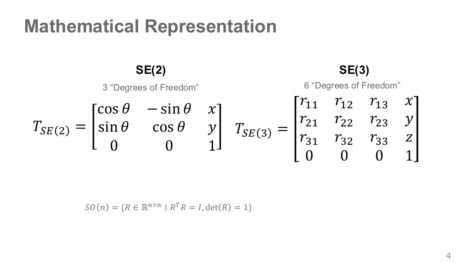
Rotation changes the directions of coordinate axes, while translation changes the origin’s position. A homogeneous transformation matrix combines both operations in one matrix product. The planar transformation below converts a point expressed in frame into frame .
Explore the symbols and calculation Planar homogeneous transformation: rotate and translate a point in frame to express it in frame
Read the equation in words
Rotate the point coordinates first, then add the displacement between origins to express the point in another frame. This does not create two separate physical points.
Understand each symbol
- A homogeneous transform converting coordinates from frame to frame .
- Homogeneous coordinates of a point in frame , with a final component of 1.
- The rotation angle in this coordinate transformation, distinct from the symbol for learned weights.
- Planar horizontal/vertical displacements or tool-tip coordinates. Specify the units and reference frame.
Follow the calculation
- Append 1 to the point to combine rotation and translation in one matrix product.
- Multiply the matrix by the point. Evaluate rotation sines and cosines using radians.
Check with a small example
After a 90° rotation and a translation of 2 to the right, rotates to and translates to .
An illustrative example for understanding the equation.
The upper-left 2×2 block is rotation, and in the rightmost column is translation. Extending a point to combines the two operations in one product. The tilde denotes homogeneous coordinates, with a final coordinate of 1. In three dimensions, the rotation block is 3×3 and the complete matrix is 4×4.
For example, rotate frame counterclockwise by 90° relative to and place its origin at . Point in is then in . The same pair of numbers does not identify the same location in different frames.
A rotation matrix satisfies and . The first condition preserves lengths and angles; the second excludes reflections. Nine matrix entries do not give orientation nine degrees of freedom. Three-dimensional rotations satisfying these constraints have three degrees of freedom.
In the three-dimensional expression, the upper-left rotation block expresses the directions of the three new coordinate axes in the original frame. Each axis has unit length and must be perpendicular to the others, so the entries cannot be chosen independently. The zeros and one in the last row add no new translational freedom; they let rotation and translation share a matrix operation. Matrix dimensions count the numbers used in a representation; degrees of freedom count independently specifiable motion variables.
#P006 · Converting sensor coordinates to robot coordinates
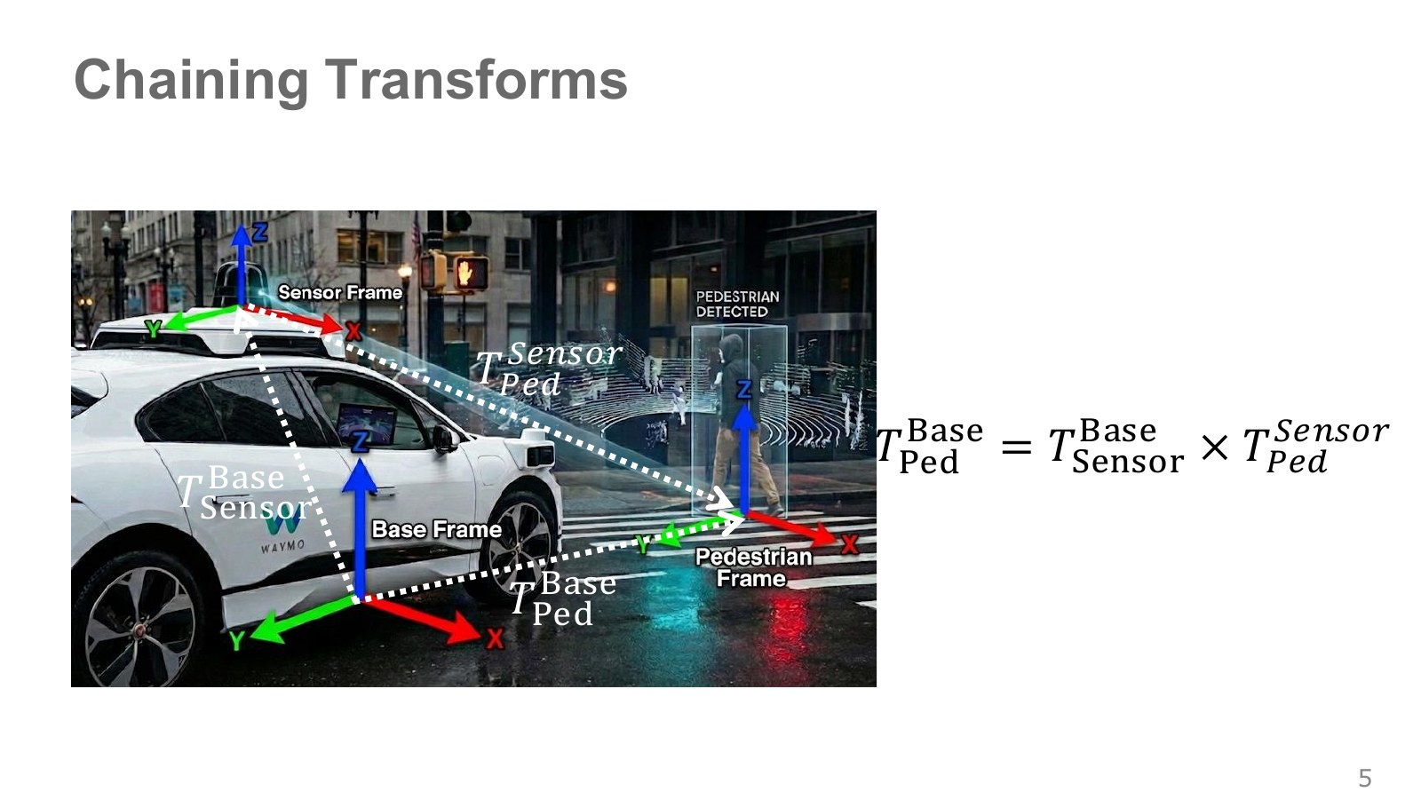
When a roof-mounted sensor detects a pedestrian, it reports a sensor-relative position—such as a distance of several ahead of the sensor. The driving controller may instead use the vehicle’s center as its reference. The two frames can differ in origin and axis directions, so passing the numbers through unchanged can point to the wrong place. The sensor’s relative position and orientation are needed to express the same pedestrian in the body frame. Connecting coordinate frames, 5:37–7:09.
A roof-mounted LiDAR reports a pedestrian in its sensor frame. Choosing an avoidance motion in the vehicle frame requires transforming those coordinates using the mounting position and orientation. Estimating that transform is extrinsic calibration. If the sensor moves, an unchanged point can appear to have changed position in the computed coordinates.
Explore the symbols and calculation Compose the transformations from pedestrian to sensor and sensor to robot reference frame
Read the equation in words
To express the pedestrian in the robot frame instead of the sensor frame, multiply transforms in an order that matches intermediate frames. Changing the matrix order changes the result.
Understand each symbol
- A transform converting sensor coordinates into robot-base coordinates.
- A transform expressing the pedestrian frame's position and orientation in the sensor frame.
Follow the calculation
- Use the rightmost transform to express the pedestrian in sensor coordinates.
- Apply the left transform to obtain robot-frame coordinates, checking that the adjacent frame names match.
Check with a small example
With no rotation, a sensor 1 m ahead of the robot and a pedestrian 3 m ahead of the sensor put the pedestrian 4 m ahead of the robot.
An illustrative example for understanding the equation.
Here, the superscript is the destination frame and the subscript is the source frame. Applying the rightmost transformation first matches the intermediate sensor frames. Reversing the order generally produces a different result. A robot arm uses the same principle when chaining base, shoulder, elbow and wrist transformations.
Determining the relationship between sensor and base is one role of extrinsic calibration. The Modern Robotics video and script on homogeneous transformations (video, 1:51–2:49) also explains coordinate representations and transformation composition. Before multiplying matrices, write down the units and the direction of each transform.
To reverse a transformation, is negating the translation enough? Following the frame explanation in Modern Robotics, 1:24–2:49 shows that the inverse rotation must be applied too. The inverse of a three-dimensional transform is:
Explore the symbols and calculation An inverse transform transposes the rotation and applies inverse rotation to the translation vector too
Read the equation in words
This reverses a rigid transformation. Negating translation alone is insufficient; the inverse rotation must also act on it.
Understand each symbol
- A rotation matrix describing rigid-body orientation, distinct here from the uppercase symbol for a reward sum.
- The translation vector separating the frame origins. Here it is not a time index.
- The inverse matrix returning to the original frame.
- The rotation matrix with rows and columns interchanged. For a valid rotation matrix, it equals the inverse.
Follow the calculation
- Transpose the rotation matrix to obtain the inverse rotation.
- Apply inverse rotation to the original translation, then negate it and use that vector as the inverse transform's translation.
Check with a small example
Without rotation, the inverse of a 2 m rightward translation is 2 m leftward. With rotation, that displacement's direction must also be expressed in the new frame.
An illustrative example for understanding the equation.
is the translation vector, not a time variable. In the earlier example with a 90° rotation and translation , inverse-transforming in returns in . This is why transforming a known point out and back is useful when checking coordinate consistency. A position point receives a final coordinate of 1, while a pure direction vector receives 0 so that translation does not affect it.
#P007 · Articulated robots: building a body from links, joints and an end effector
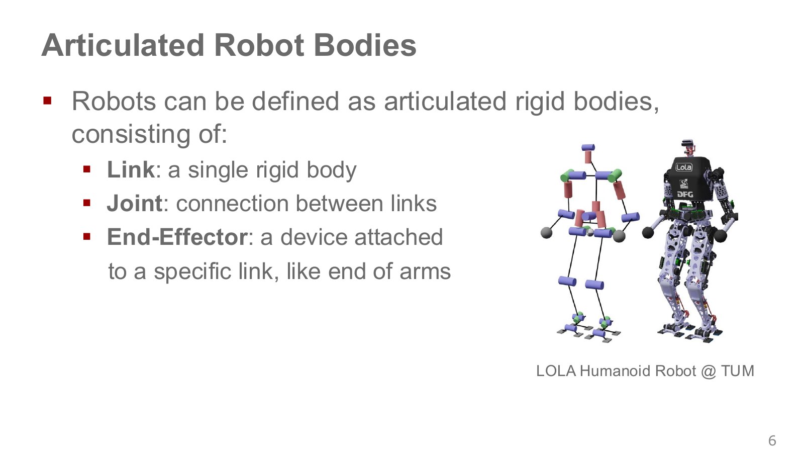
An articulated robot consists of multiple bodies connected by joints that allow their relative positions or orientations to change. Industrial arms often connect several rotational joints to move the tool tip, much as a person bends a shoulder, elbow and wrist. “Articulated” describes how the body is connected and moves, rather than a type of AI. The pictured LOLA humanoid can likewise be modeled by separating its torso, arms and legs and their connections.
A link is an individual body approximated as rigid, such as treating the upper arm and forearm as separate units. A joint is a mechanical connection permitting particular relative motions between those bodies. Bending an elbow changes the angle between the upper arm and forearm, not their lengths. An end effector is the tool at the end that interacts directly with the task object. It may be a gripper, suction tool or welding torch and can be changed to suit the task.
Changing a joint angle changes the coordinate transformation between links; multiplying the connected transforms gives the hand position. Count the joints, but also identify which links they connect and along which axes. Different link lengths or joint axes send the hand to different locations even for the same angle vector.
A robot’s fixed support is its base. The sequence of links and joints from base to tool tip is a kinematic chain. The humanoid branches from its torso into two arms and two legs, so it can be viewed as having several chains. Foot–ground contact adds motion constraints. Deciding which parts to model as rigid bodies and which connections as joints is the starting point for motion equations. Modern Robotics on rigid bodies, links and joints.
#P008 · Reading the joint structures of Franka and SO-101
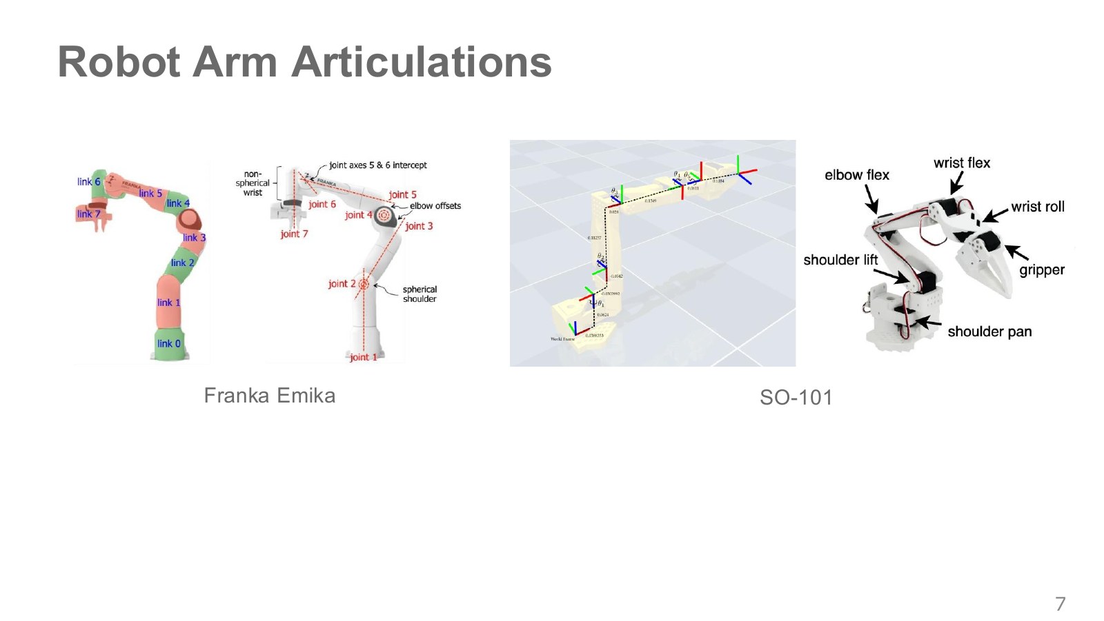
In the Franka diagram, link 0 lies at the support, while links 1 through 7 follow the arm. Joints 1 through 7 identify rotational axes between neighboring bodies. Turning the first joint moves the whole connected arm above it; turning the last mainly changes the wrist pose. Offsets between axes also change how rotation affects tool-tip position. The model therefore includes axis directions and distances between axes as well as body lengths.
On the SO-101, shoulder pan rotates the shoulder left and right; shoulder lift raises it; elbow flex bends the elbow; wrist flex bends the wrist; and wrist roll twists about the wrist’s longitudinal axis. The gripper drive opens and closes the fingers. The colored coordinate axes attached to each link provide references for calculating position and orientation. Connecting the joint values through these frames gives the gripper’s location and direction.
Count arm degrees of freedom separately from gripper opening and closing. Variables setting the tool’s three-dimensional position, its orientation and its opening width serve different roles. A six-element joint vector does not necessarily provide six-degree-of-freedom spatial pose control.
Franka has seven arm joints. In the SO-101 diagram, five arm joints move and orient the gripper, while another drive opens and closes it. Six drive values therefore do not establish independent control over all six spatial position and orientation components. Changing gripper width does not replace a wrist-tilt degree of freedom. This distinction matters when judging whether different arms can perform the same goal.
#P009 · Changing the grasping tool changes the action space
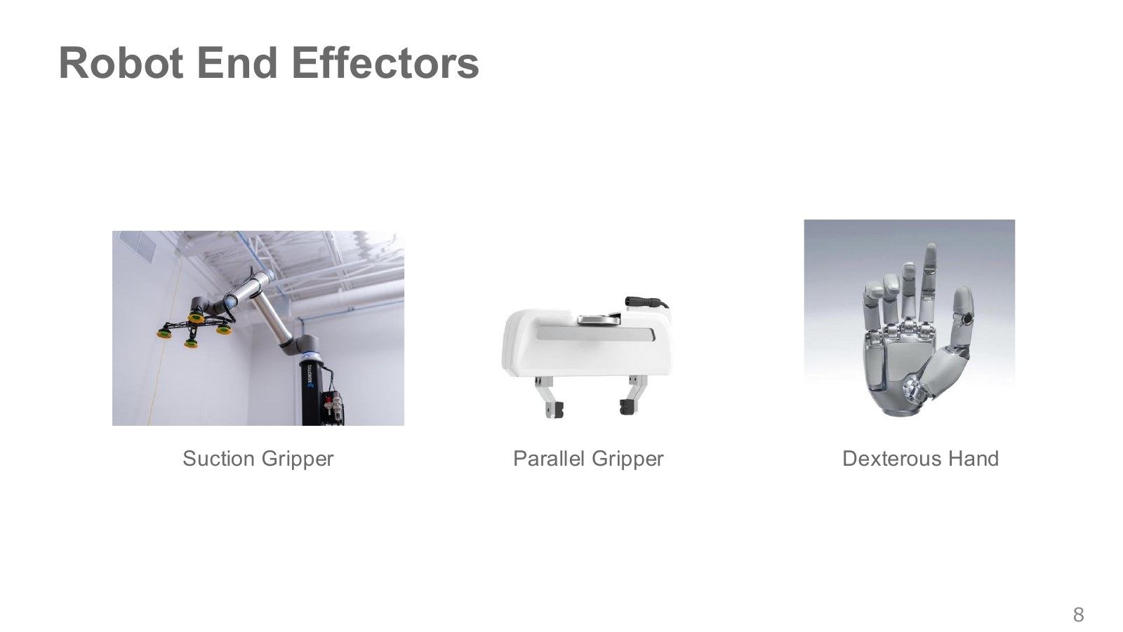
A suction gripper may have a command to switch vacuum on or off; a parallel gripper controls opening width or force. An articulated hand requires coordinating multiple finger joints. Changing the contact mechanism changes both the required precision and the dimensionality of the actions to learn.
If the command only switches suction on or off, it has two choices and can be represented as a binary action. Video, 9:09–10:35. This does not make the arm position and orientation used to bring the suction tool over an object binary. A single policy can combine continuous arm commands with a discrete grasp command.
A suction tool holds an object through a pressure difference between its cup and the object’s surface. The material and gaps affect whether it seals, so activating suction does not establish a successful grasp. A parallel gripper moves two opposing fingers to press on an object; contact and sufficient force matter alongside width. An articulated hand can adjust multiple contacts to handle complex shapes, but requires estimating and controlling more finger joints and contact states. The tool choice changes both what must be observed and what must be commanded.
If the fingers of a parallel gripper move symmetrically, one opening-width variable specifies their configuration. Two fingers do not necessarily mean two independent degrees of freedom. An articulated hand, by contrast, can have over 20 degrees of freedom, requiring choices about each finger as well as the overall grasp. A larger policy output dimension means more independent choices of this kind. Tools and action dimensions, 9:29–10:35.
#P010 · A joint constrains which motions are allowed
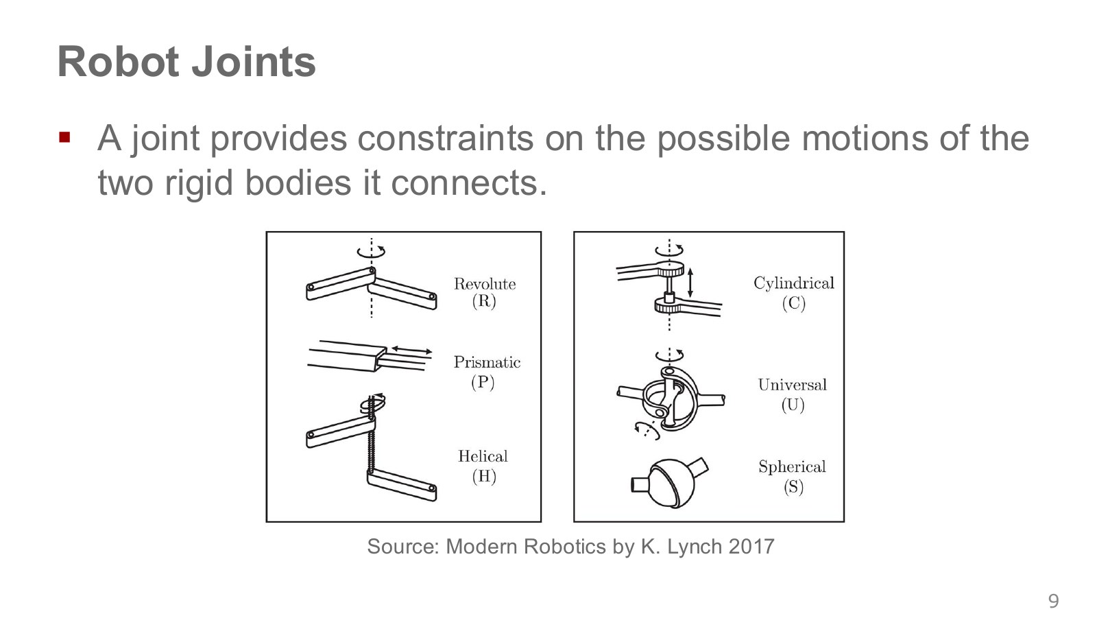
Two unconstrained rigid bodies moving relative to one another require three position and three orientation variables in space. A revolute joint allows rotation about one axis and prevents the other relative motions. A prismatic joint allows translation along one axis.
Think of a door hinge. The door rotates about the hinge axis, but does not freely detach sideways or slide along that axis. A joint enables certain motions while preventing others. A constraint is a condition tying motion variables together so they cannot be chosen independently.
The six joints in the diagram can be distinguished as follows. Degrees of freedom count the variables that can change independently between two links. Modern Robotics on joint types and degrees of freedom.
| Joint | Permitted relative motion | Degrees of freedom | An intuitive example |
|---|---|---|---|
| Revolute () | Rotation about one axis | 1 | One angle changes, as in a door hinge. |
| Prismatic () | Translation along one axis | 1 | One distance changes, as with a slider on a rail. |
| Helical () | Rotation and translation along the same axis coupled at a fixed ratio | 1 | Turning a screw advances it by its specified pitch. |
| Cylindrical () | Independent rotation and translation along the same axis | 2 | Rotation and sliding distance can be set separately. |
| Universal () | Rotation about two intersecting axes | 2 | Imagine a cross-shaped connection bending in two directions. |
| Spherical () | Rotation in three directions about one point | 3 | A ball joint changes orientation while retaining its center. |
A helical joint rotates and translates, but the two motions are coupled, giving one degree of freedom. A cylindrical joint permits those motions independently and has two. That is why we ask how many motion variables can be chosen independently, rather than simply counting visible motors. Passive joints and drives coupling several joints also mean that motor count and kinematic degrees of freedom need not match.
#P011 · Distinguishing degrees of freedom from state dimension
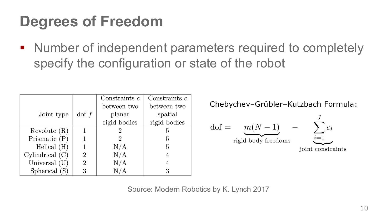
Degrees of freedom (DoF) count the independent variables needed to specify a robot’s geometric configuration. The slide introduces a calculation that subtracts joint constraints from the rigid bodies’ original freedoms.
Explore the symbols and calculation Subtract the independent constraints imposed by joints from the rigid bodies' degrees of freedom
Read the equation in words
Start with the freedoms of the rigid bodies and subtract independent motions prevented by joints. A body fixed to the ground is not counted as freely moving.
Understand each symbol
- The degrees of freedom of one rigid body: 3 in the plane and 6 in space.
- The total link count, including the fixed body.
- The total joint count and the number of independent motions constrained by joint .
- Add every term over the indicated range, computing one term and repeating through the end of the range.
Follow the calculation
- Exclude one fixed body and multiply the remaining body count by the rigid-body freedoms for that spatial dimension.
- Subtract all independent joint constraints. Overlapping constraints invalidate direct use of this simple count.
Check with a small example
A planar 2R arm has three bodies including the base and two revolute joints, giving degrees of freedom.
An illustrative example for understanding the equation.
is 3 for a planar rigid body and 6 for a spatial one. counts links including the fixed base, counts joints, and is the number of relative freedoms removed by each joint. The calculation assumes independent constraints; direct substitution can fail for special mechanisms. A planar serial 2R arm has three links and two revolute joints, giving .
Here, configuration and dynamical state are different. If a two-DoF arm’s configuration consists of two joint angles, predicting its motion may also require two joint velocities. An arm moving quickly and a stationary arm evolve differently even at the same angles. This distinction becomes important when defining an MDP state later.
The table’s constraints column expresses the same calculation from the other side. Two spatial rigid bodies have six relative degrees of freedom; a revolute joint leaves one, imposing five motion constraints. In the plane, there are three relative freedoms, so the same revolute joint imposes two constraints. Including the base in the link count lets us count its joint to the first moving link in the same way as other joints. Closed-loop mechanisms can have overlapping constraints, so their independence requires particular attention.
#P012 · Configuration space and the periodicity of joint angles
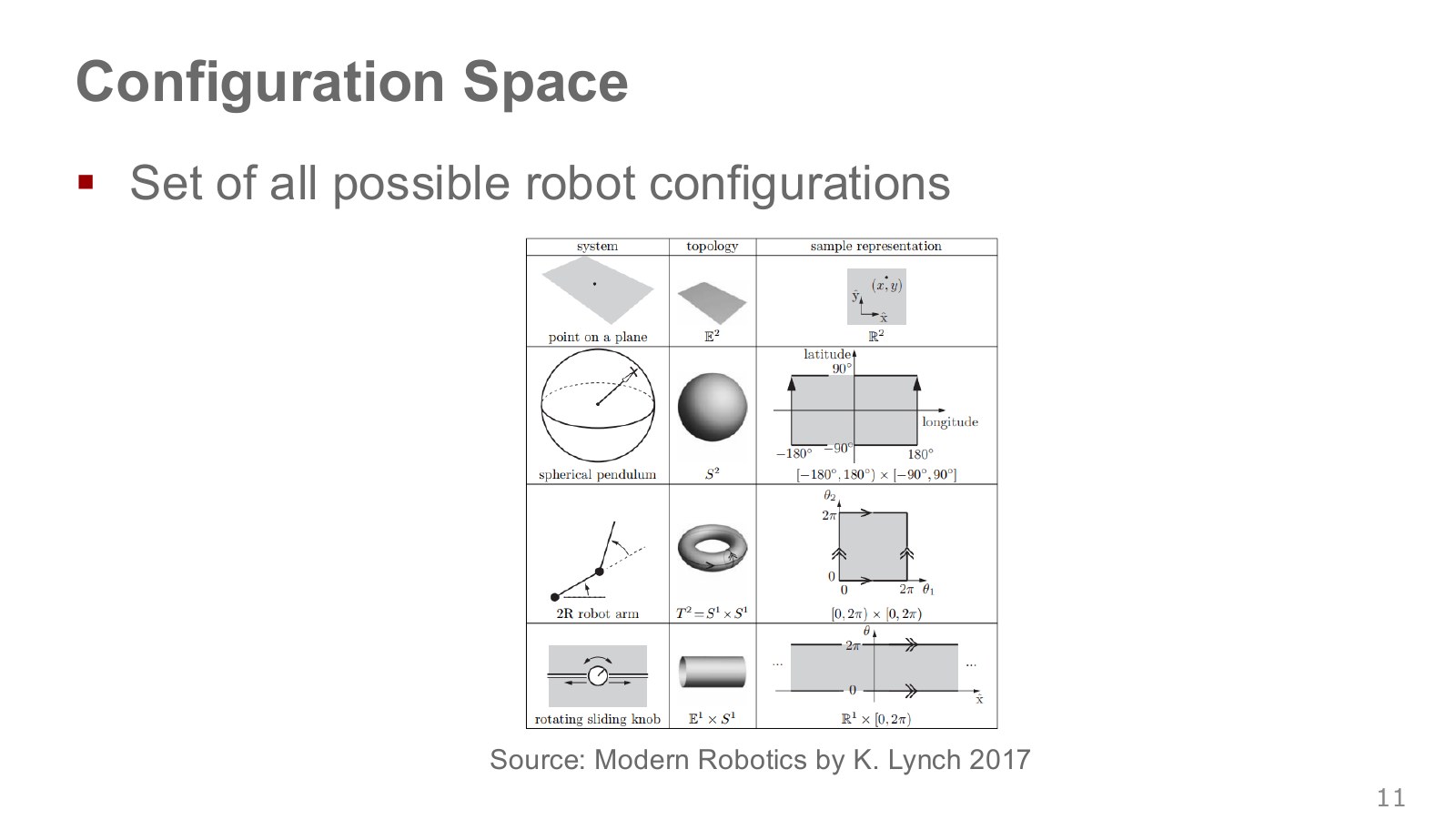
Configuration space, or C-space, is the set of all possible joint configurations. One configuration of a 2R arm is an angle pair : a point in this space describes one arm configuration. This differs from the space in which we plot the hand’s position above a table.
An unrestricted revolute joint returns to the same configuration after one full turn. The ideal configuration space of two such joints is the product of two circles—a torus. Real joint limits restrict the feasible subset.
At an angle’s numerical boundary, simple subtraction may miss the shorter physical rotation. As an illustration, moving from 359° to 1° has a short difference of +2°, rather than the −358° obtained by direct subtraction. Mechanical limits or cables may prevent crossing that boundary, in which case the short route is not allowed either. Representing angles with in a neural-network input is one way to capture periodicity.
The other examples become clearer when we separate variable count from the shape of a space. A point in a plane needs two position coordinates, yielding a plane of possible positions. The endpoint of a fixed-length spherical pendulum stays the same distance from the center and moves on a sphere’s surface, described by two direction variables. A handle that both slides and rotates needs one displacement and one angle, producing a cylinder-like space combining a line and a circle. Having two variables does not make all these spaces the same plane. Configuration-space shapes and coordinate representations.
#P013 · Workspace: the places a hand can reach
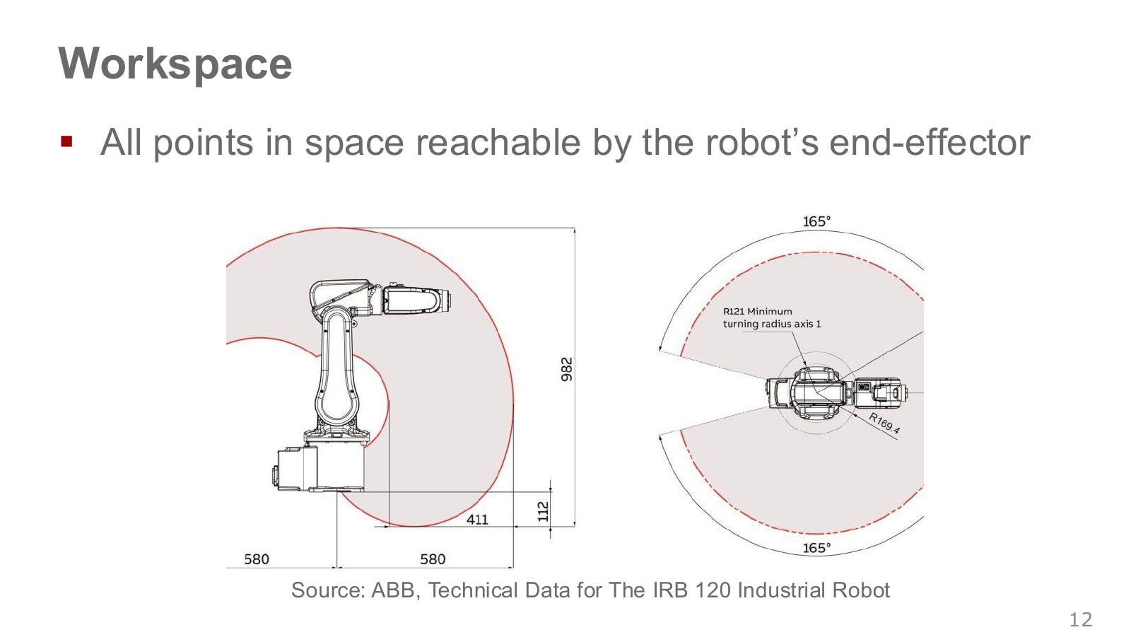
Here, workspace means the set of positions the end effector can physically reach. Think of the reach envelope around the base in the ABB diagram. Its coordinates have a different meaning from the joint angles of C-space.
A point inside that envelope may still be unreachable at the desired orientation or through an obstacle-free approach. A cup being within arm’s reach does not guarantee a feasible grasp. Wrist orientation, joint limits and elbow–table collisions also need checking.
Consider an ideal planar 2R arm with link lengths . Ignoring joint limits and self-collision, the distance between tool tip and base lies between and . With two 1 m links, positions within a 2 m radius are reachable, but not every desired hand orientation can be achieved at every point.
The two C-space coordinates in this example are the joint angles; the two workspace coordinates are the hand’s planar position. Equal dimension does not make them the same space. Forward kinematics connects them, and that relationship also explains multiple inverse-kinematics solutions. The explanation in ETH, 13:58–14:41—the cup is seen in workspace, while execution occurs in joint configuration—can be read through this example.
The ABB side and top views show sections or projections of the same robot’s reach envelope from different directions. Joint limits and link lengths make some points around the base feasible and others infeasible. The shaded region helps assess reachability first; the orientation of an approach with a particular tool still needs separate checking. Some literature includes end-effector orientation in its definition of workspace. Here we retain the narrower convention of reachable positions. Task space and workspace.
#P014 · From physical obstacles to forbidden regions in joint space
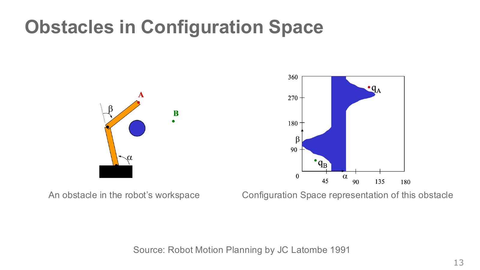
The blue circle on the left is a physical obstacle. The plot on the right colors the joint-angle combinations at which the arm collides with it. It is not a direct copy of the obstacle’s shape: it is the result of checking the shape of the entire arm and its collisions for each angle combination.
A link in the middle of the arm can touch an obstacle even when the tool tip lies outside it. Conversely, bending the elbow the other way can avoid a collision at the same tool-tip position. Drawing a straight line for the hand and finding a safe path for the whole robot are therefore different problems.
The horizontal and vertical axes of the right-hand plot are joint angles, not distances across a table. Picking one point fixes both angles and therefore the entire arm shape in the left-hand space. If that shape touches the obstacle, the point is colored blue. The curved or broad blue region comes from multiple angle combinations producing collisions, not from deforming the obstacle. Even if start and goal are both in white regions, straight-line interpolation between their joint angles collides if it passes through blue.
#P015 · Path planning finds a connection around forbidden regions
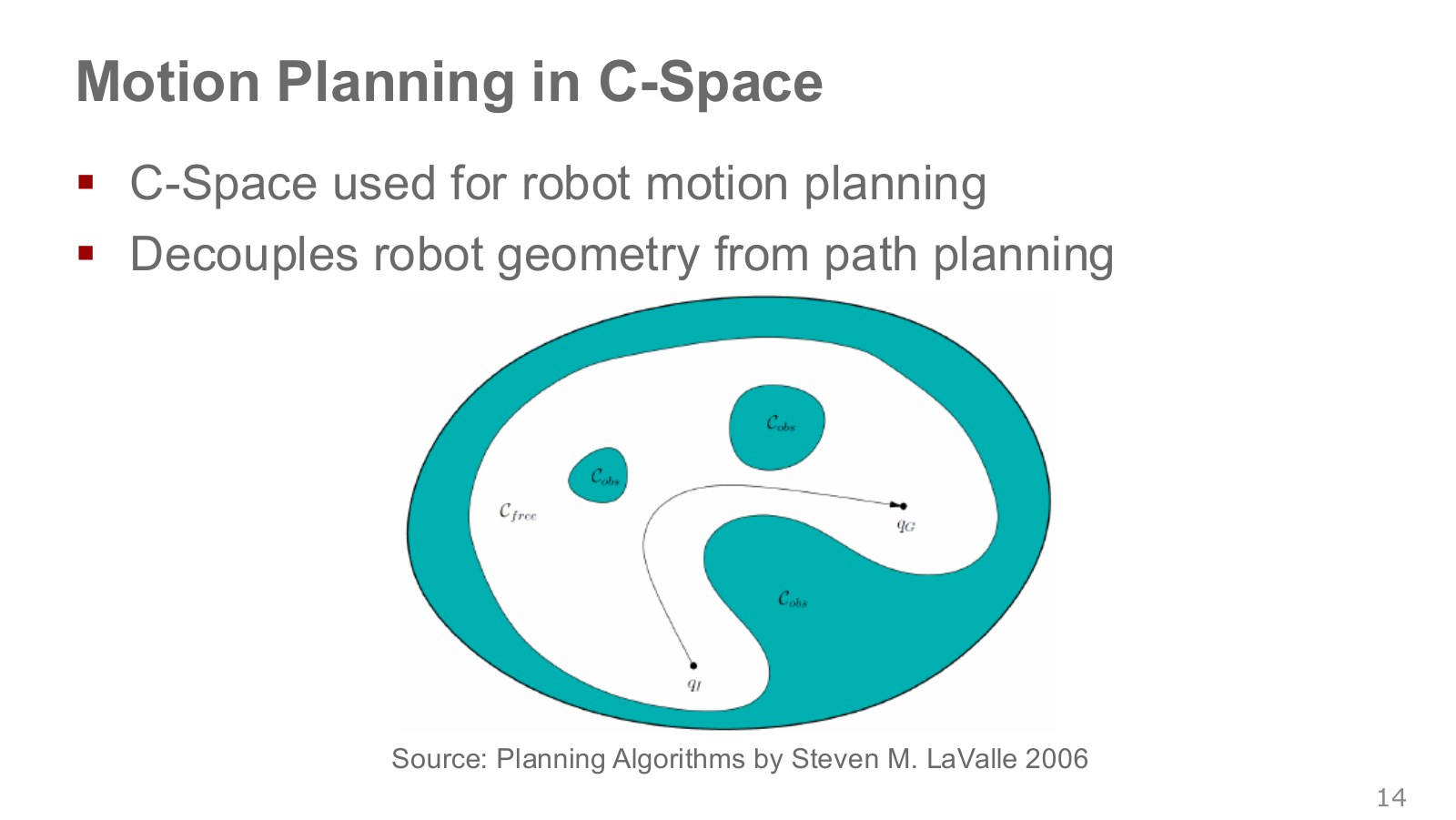
Representing the robot’s start and goal configurations as points in C-space turns path planning into connecting those points within the collision-free region. Collision checking accounts for the robot’s full thickness and its relationship to obstacles; the path itself is a continuous sequence of configurations.
As joint count increases, the space of angle combinations grows in dimension, making it difficult to precompute every forbidden region. Discussion, 14:44–16:42. This does not mean discarding geometric planning. Sampling-based planners can check collisions at selected configurations, and learned policies still need constraint handling and collision checks during execution. Keep the distinction that a path says where to move, while a trajectory says when and how.
The turquoise region contains forbidden configurations; the white region contains configurations free of collision. A curve connecting start and goal must remain in white. Each point on the curve is one arm configuration, and following the curve changes configurations in sequence. The figure still has no schedule specifying which point is crossed at which time. Adding that timing produces the trajectories and control commands discussed later.
#P016 · Task space: coordinates that express the goal naturally
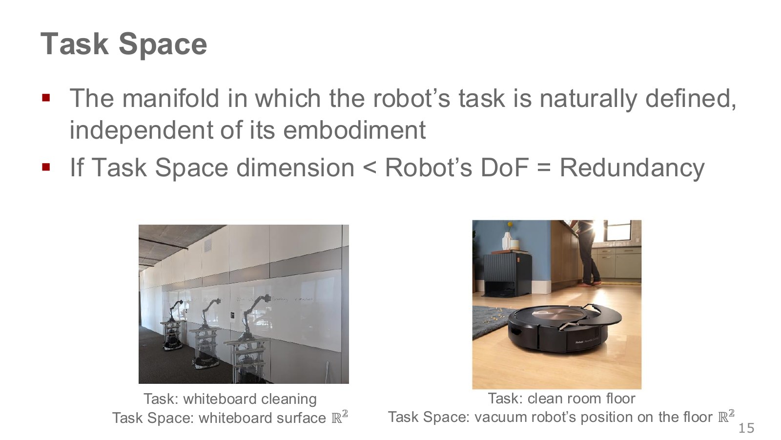
Task space is a space of variables natural for describing the work. A whiteboard-wiping location can use two coordinates on the board, and a floor-cleaning location can use two coordinates on the floor. It is a starting point for expressing the goal independently of the robot’s joint structure.
That does not mean two numbers alone suffice for control. If the eraser must maintain its orientation and force against the board, those conditions become additional constraints. The task dimension depends on what we hold fixed and what we leave free.
The same goal—wipe a particular mark on a board—can be given to a five-joint or seven-joint arm, but the joint angles needed to touch it differ. Think of task space as where we describe the work, configuration space as where we describe that robot’s body configuration, and workspace as where its hand can reach. This makes the directions of FK and IK easier to follow.
#P017 · Why the elbow can move while the hand stays still
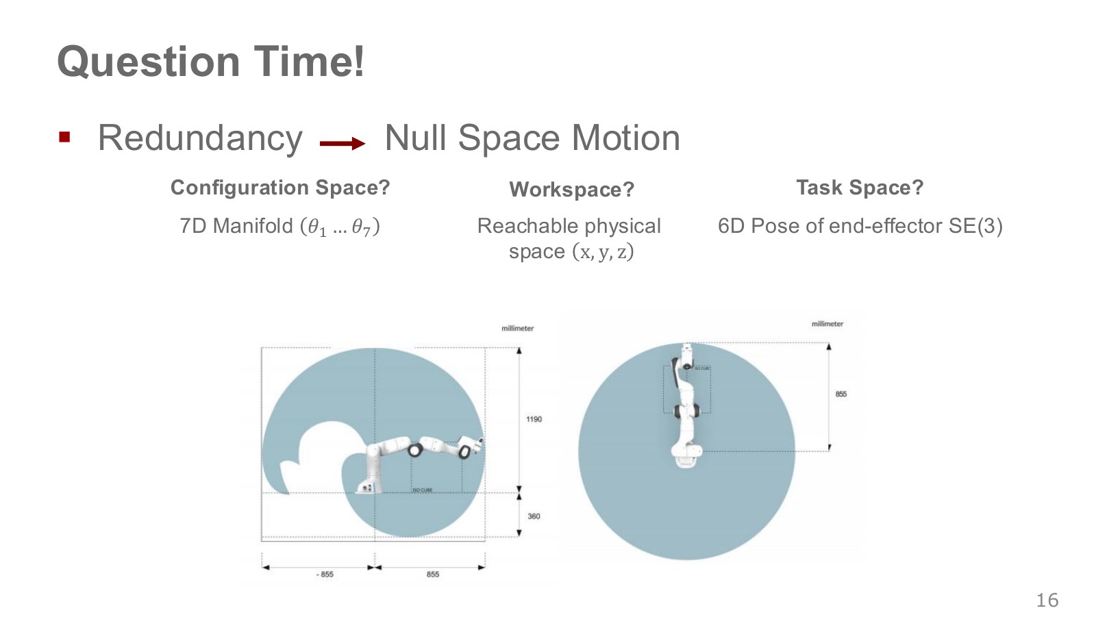
Franka’s arm configuration is seven-dimensional, while the hand’s spatial position and orientation are locally six-dimensional. In an ordinary configuration, multiple joint configurations can produce the same hand pose. This is kinematic redundancy.
In the Franka example, the elbow can move while the cup’s position and orientation remain fixed. This freedom can help avoid nearby objects without tilting the cup. The available directions and range depend on the current configuration and joint limits.
Try moving your elbow while holding a coffee cup in place without tilting it. There is room to change the rest of the arm while retaining the hand’s position and orientation. Example, 18:20–19:17. In differential terms, null-space motion is joint motion that leaves the current task output unchanged. It can help avoid joint limits or maintain clearance from obstacles. Simple dimension counting can change at singular configurations or under additional contact constraints.
Writing tool-tip position as , its small change is approximated by . A joint change satisfying therefore leaves the tool tip stationary to first order. The null space consists of directions producing zero in that equation. One finite movement need not hold the tool tip exactly fixed, so actual control recomputes at the updated configuration while maintaining the target.
Having room to move the elbow does not guarantee that every obstacle can be avoided. Without sufficient clearance or joint range, even a redundant arm may have no collision-free solution.
Earlier, workspace meant reachable positions, while task space meant the coordinates expressing the goal. The six compared with seven here is the local dimension of the task of controlling the hand’s full position and orientation. This is not a comparison of the physical reach envelope’s size or volume with joint space. At an ordinary configuration where the Jacobian spans all six independent task directions, one remaining direction of joint motion may leave hand pose unchanged.
#P018 · Forward kinematics: from joints to tool tip
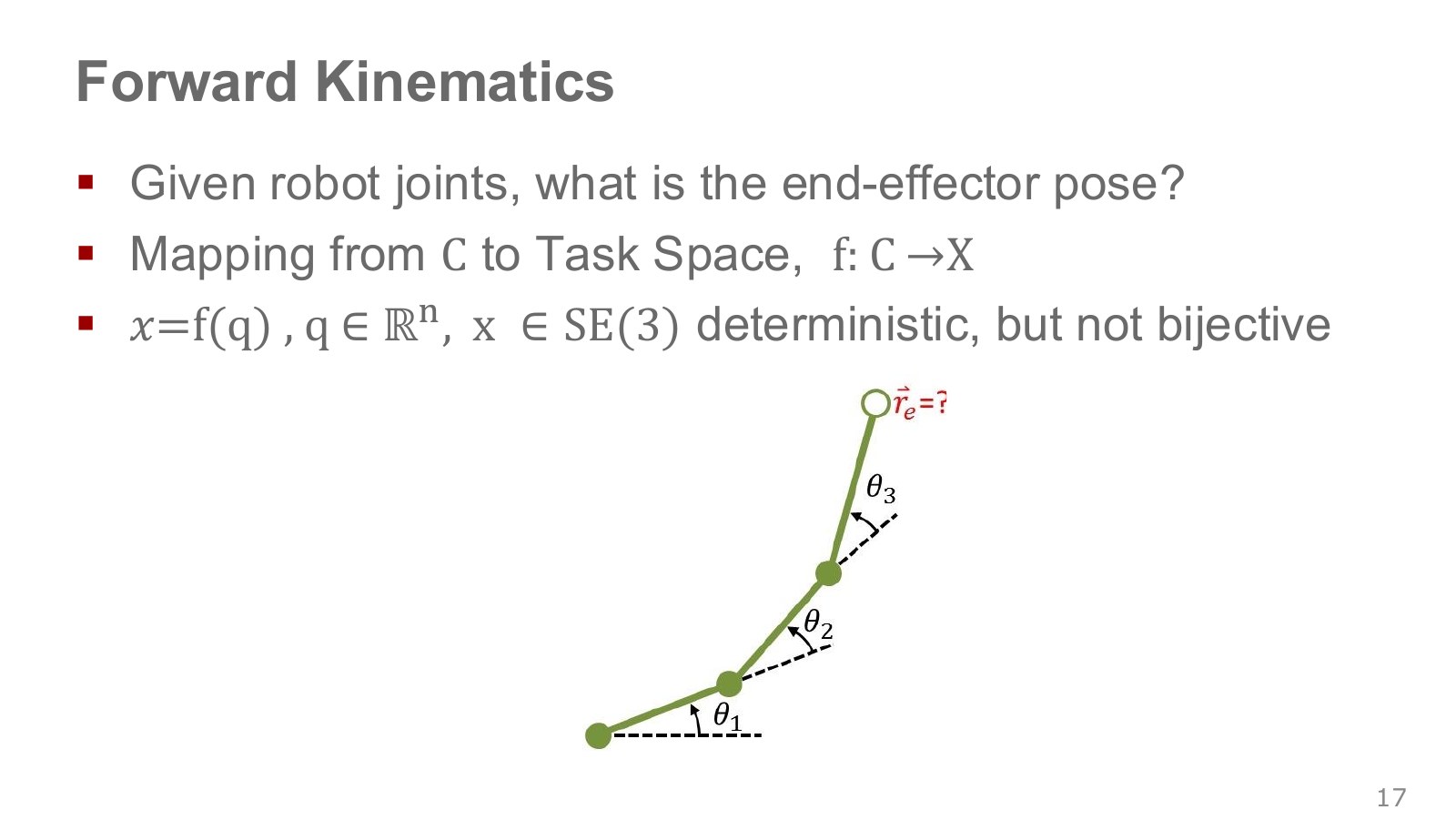
Forward kinematics (FK) computes the end effector’s position and orientation from a known joint configuration . Given a model with fixed link lengths and joint axes, each configuration produces one hand pose, written as .
For a planar 2R arm with link lengths and joint angles , the tool-tip position is given below. This separate example illustrates the principle.
Explore the symbols and calculation A planar 2R arm's tool-tip position is the sum of its two rotated link-length vectors
Read the equation in words
Add the second link's extension to the first link's endpoint. The second link's direction is the sum of the first and second joint angles.
Understand each symbol
- The first and second relative joint rotation angles. Both contribute to the second link's overall direction.
- The two link lengths: fixed body dimensions, not angles changing during rotation.
- Planar horizontal/vertical displacements or tool-tip coordinates. Specify the units and reference frame.
Follow the calculation
- Multiply each link length by the cosine of its direction for the horizontal component and by the sine for the vertical component.
- Add the horizontal components and the vertical components separately.
Check with a small example
With two 1 m links and both angles zero, the tool tip is . Turning only the first angle to 90° gives .
An illustrative example for understanding the equation.
The second link’s direction is , rather than , because the second angle is measured relative to the first link. With 1 m links and , the tool tip is at . FK is distinct from dynamics, which computes quantities such as forces and accelerations.
In the arm diagram, the first angle sets direction relative to the base; later angles describe bending relative to preceding links. Accumulating those angles and moving along each link locates the endpoint. Specifying all joint values determines one modelled tool pose, so FK is deterministic. But different joint values can produce the same tool-tip position, so it is not one-to-one. Having a determined forward result and a unique inverse solution are different properties.
#P019 · Inverse kinematics: from a tool-tip goal to joints
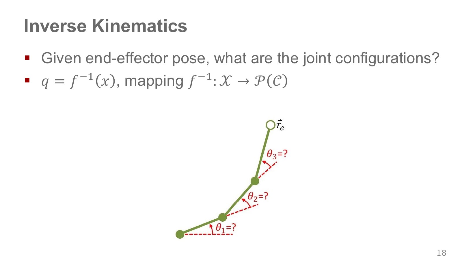
Inverse kinematics (IK) finds joint configurations that produce a desired hand position and orientation. When a policy outputs tool-tip targets, IK connects those targets to joint commands.
For the 2R arm above, also produces tool-tip position . Different elbow configurations can reach the same position. Because the target here specifies position only, the two solutions need not have the same tool orientation. Including orientation changes the solution set. Thus should not be read as a simple inverse function returning one answer.
The red question mark indicates that the endpoint is known but the joint angles are not. Given link lengths and joint structure, we must find angle combinations that reach the goal. The original expression uses set notation to show that an answer need not be one numerical vector: there may be multiple solutions, or an empty set when the target is unreachable. Reading FK backward does not always reduce the problem to one matrix inversion.
#P020 · IK can have multiple solutions, no solution or a local solution
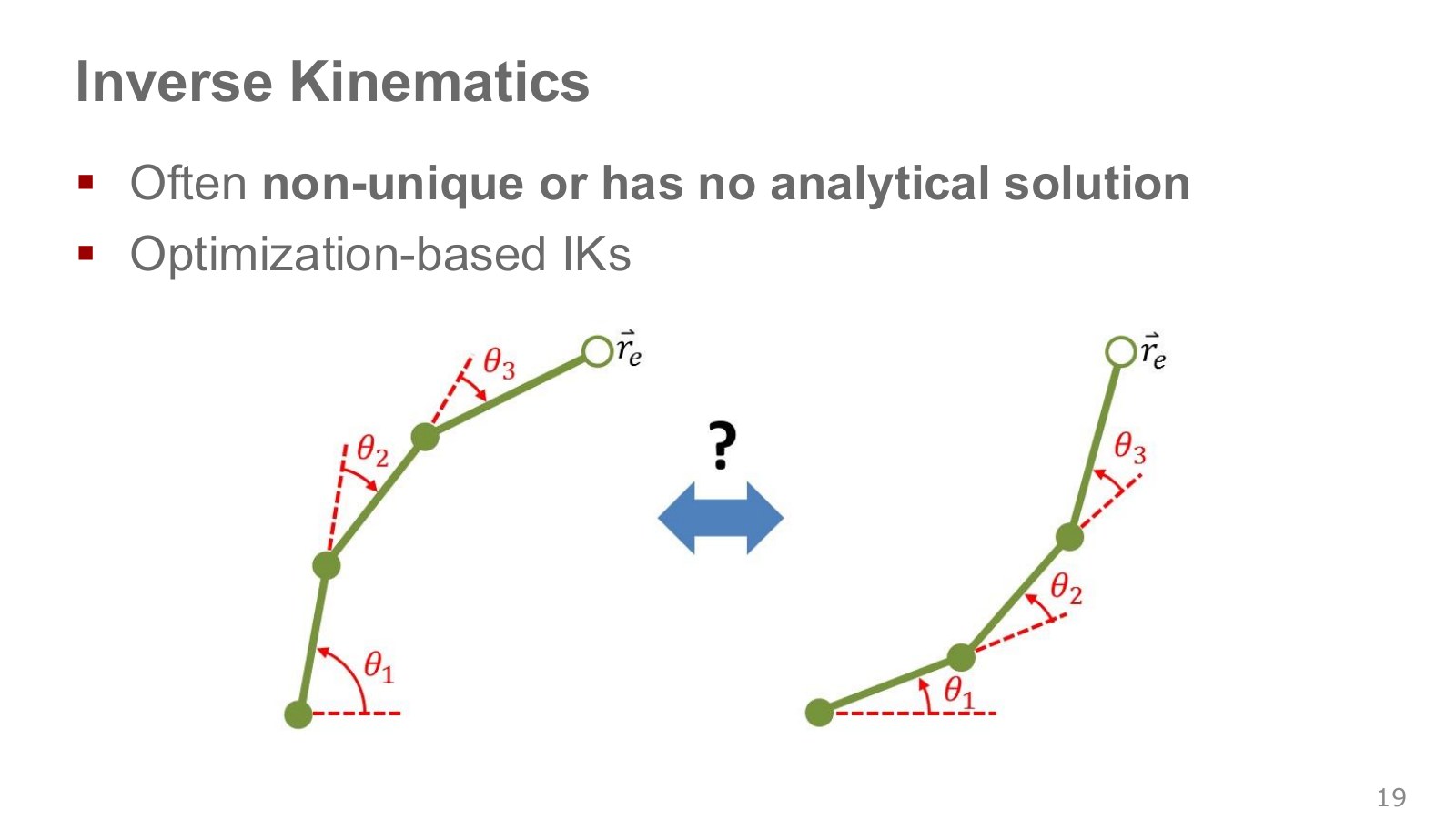
A goal outside the reach envelope has no exact solution. Even a reachable goal may become infeasible after joint limits or collisions are considered. Multiple solutions require a selection criterion, such as proximity to the current configuration or clearance from obstacles.
When a direct formula is difficult to obtain, IK can be solved as an optimization problem that repeatedly changes joint values to reduce the tool-tip error. Numerical IK, 20:42–21:30. The initial configuration and step size can change the numerical outcome. A small final tool-tip error does not establish a collision-free path to it.
Modern Robotics on numerical IK, 1:55–2:19 and 4:24–4:42 explains how initial estimates can lead to different solutions and how a small gradient can produce an excessively large update. When following successive tool-tip targets, we can therefore use the previous solution as the next target’s initial estimate instead of restarting from arbitrary joint angles each time.
When moving a hand in 1 cm increments, neighboring targets are close, so the previous configuration may be a good starting point for the next solution. Joint limits, singularities or new obstacles can break that continuity. Check whether the target was reached alongside the initialization, stopping tolerance and iteration limit.
#P021 · Using the Jacobian to move toward a target in small steps
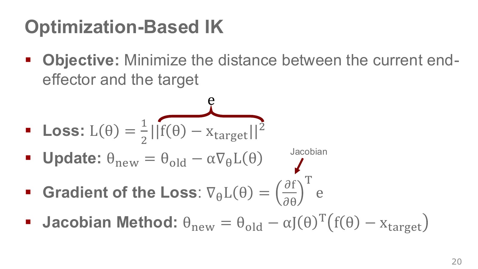
First consider position targets only, expressing and target as vectors in the same Euclidean coordinates. Writing the slide’s consistently as joint variable gives the following.
Explore the symbols and calculation Reduce squared position-IK error by gradient descent using the Jacobian transpose
Read the equation in words
Adjust the joints in small increments to reduce squared tool-tip distance to the target. The Jacobian transpose maps tool-tip error back into a joint-update direction.
Understand each symbol
- The joint configuration at optimization iteration . The subscript is an iteration index here, not a joint index.
- The forward-kinematics function mapping joint configuration to tool-tip position.
- The desired tool-tip position. The asterisk marks a target in this equation.
- The error vector obtained by subtracting target position from current tool-tip position.
- A loss quantifying the difference between a prediction and a target. Learning or optimization aims to reduce it.
- The Jacobian matrix describing tool-tip change for a small joint change.
- The learning rate setting the update size. A large value can move faster but destabilize the iteration.
- The squared length obtained by squaring and summing all vector components. It combines coordinate-wise errors into one nonnegative quantity.
Follow the calculation
- Compute tool-tip position and error from the current joint values.
- Multiply error by the Jacobian transpose, subtract the result scaled by the learning rate, and recompute at the new position.
Check with a small example
In a one-dimensional example where tool position equals the joint value, current 2 and target 3 give error −1. With learning rate 0.1, the next joint value is .
An illustrative example for understanding the equation.
is the Jacobian. It describes the direction and amount of tool-tip movement produced by a small joint change. With task coordinates and joint variables, has shape , and has the same dimensions as the joint vector. is the step size controlling each update; is the optimization iteration index.
Because the error is , the update moves in the negative-gradient direction. This is gradient descent using the Jacobian transpose, distinct from directly applying an inverse or pseudoinverse. Including hand orientation requires an orientation-error representation and relative position/orientation weights, rather than simply subtracting SE(3) matrices.
After an update, recompute FK and the Jacobian at the new joint values. Continue until the error is sufficiently small or the iteration limit is reached. One calculation does not teleport the tool tip to the goal. Update equation, 21:31–22:19. The executable example below also checks this gradient against numerical differentiation.
Even with the same Jacobian, the update depends on what we want to compute. Modern Robotics, 2:21–4:23 treats tool-tip error as a local linear problem and solves it with a pseudoinverse. To remain consistent with this section’s error and its sign, define the desired change toward the target as .
Explore the symbols and calculation Apply a pseudoinverse or damped least-squares matrix to target-directed error to obtain a joint increment
Read the equation in words
These are two ways to convert desired tool-tip movement into joint movement. Damped least squares moderates excessive increments where inverse calculations become unstable.
Understand each symbol
- The Jacobian matrix describing tool-tip change for a small joint change.
- The identity matrix: diagonal entries are 1 and others 0. Multiplying a compatible vector by it leaves the vector unchanged.
- Small changes in joint values and tool-tip position, respectively.
- A pseudoinverse providing a least-squares inverse calculation even without a square invertible matrix.
- A positive damping magnitude. Larger values suppress joint changes more, but can reduce accuracy in the desired tool movement.
Follow the calculation
- Specify a small desired tool-tip displacement.
- Multiply by the pseudoinverse or use the matrix formed with positive damping to calculate joint changes. Both are local calculations around the current pose.
Check with a small example
In one dimension, Jacobian 2 and desired displacement 0.1 give pseudoinverse increment 0.05. With damping 1, the result is .
An illustrative example for understanding the equation.
is the Moore–Penrose pseudoinverse. If the local linear equation has multiple solutions, it selects the joint change with the smallest Euclidean norm; if an exact match is impossible, it minimizes the linear residual. This does not guarantee a global optimum of the nonlinear IK problem. The DLS damping factor reduces excessive updates along weak directions, and is an identity matrix sized to the task dimension.
The official NVIDIA Isaac Lab implementation offers transpose (trans), pseudoinverse (pinv) and DLS (dls) as distinct options. It takes a tool-tip position error and Jacobian, computes a joint increment, and adds it to the current joint values. This is where the equations meet code.
In a separate 2R calculation, both links were 1 m, the first joint was at 0 rad, and the desired change was −1 mm along . With DLS parameter , one linear calculation gave the following results.
| Second joint | Pseudoinverse joint-change norm (rad) | DLS joint-change norm (rad) |
|---|---|---|
| Bent at /2 rad | 0.001000 | 0.000995 |
| Nearly straight at 0.001 rad | 2.236068 | 0.000179 |
| Fully straight at 0 rad | 0 | 0 |
Near a straight configuration, exactly matching a small tool-tip change in the linear equation can demand a large joint change. DLS moderates it but may leave a tool-tip residual. At full extension, the first-order Jacobian cannot express inward motion along , so both calculations returned zero. The target is not physically impossible; the local linearization at that configuration cannot represent motion in that direction. This illustrates why a small initial bend or another search strategy may be needed. The table comes from a separate NumPy calculation of the published equations, not an Isaac Lab run.
Read the four equation lines in order. First subtract the target tool-tip position from the current FK position to form the error. Squaring and summing its components gives the loss. If the current tool tip is 2 cm beyond the target along and aligned along , the error vector is . The factor 1/2 cancels the factor 2 arising when the square is differentiated; it does not change where the loss is minimized.
Each Jacobian column describes one joint’s contribution. Hold the other joint fixed and record how the tool tip moves when one joint turns slightly, then do the same for the other. With two position coordinates and two joints, the matrix reads as follows.
Explore the symbols and calculation Jacobian of a planar two-joint arm: columns describe joint contributions; rows describe tool-tip and changes
Read the equation in words
Each column shows the direction and amount of tool-tip motion from a small rotation of one joint. Rows correspond to tool-tip coordinate components.
Understand each symbol
- The first and second relative joint rotation angles. Both contribute to the second link's overall direction.
- Planar horizontal/vertical displacements or tool-tip coordinates. Specify the units and reference frame.
- The rate of horizontal-position change when only the first joint changes and other joints remain fixed.
Follow the calculation
- Change just one joint very slightly and inspect the horizontal and vertical tool-tip changes.
- Collect the contributions as columns to obtain a matrix relating joint velocity to tool-tip velocity.
Check with a small example
If a 0.01 rad joint change moves the tool tip horizontally by 0.02 m, that derivative is approximately m/rad.
An illustrative example for understanding the equation.
The first row describes changes in and the second changes in . measures how the position changes when only the first joint angle changes slightly. Combining this matrix with the current tool-tip error determines which way to adjust the joints to reduce that error. maps tool-coordinate error into the loss gradient for each joint. The same error therefore produces different updates in a straight and a bent arm. Reading Jacobian columns as individual joint contributions.
#P022 · Finding target angles is different from reaching them physically
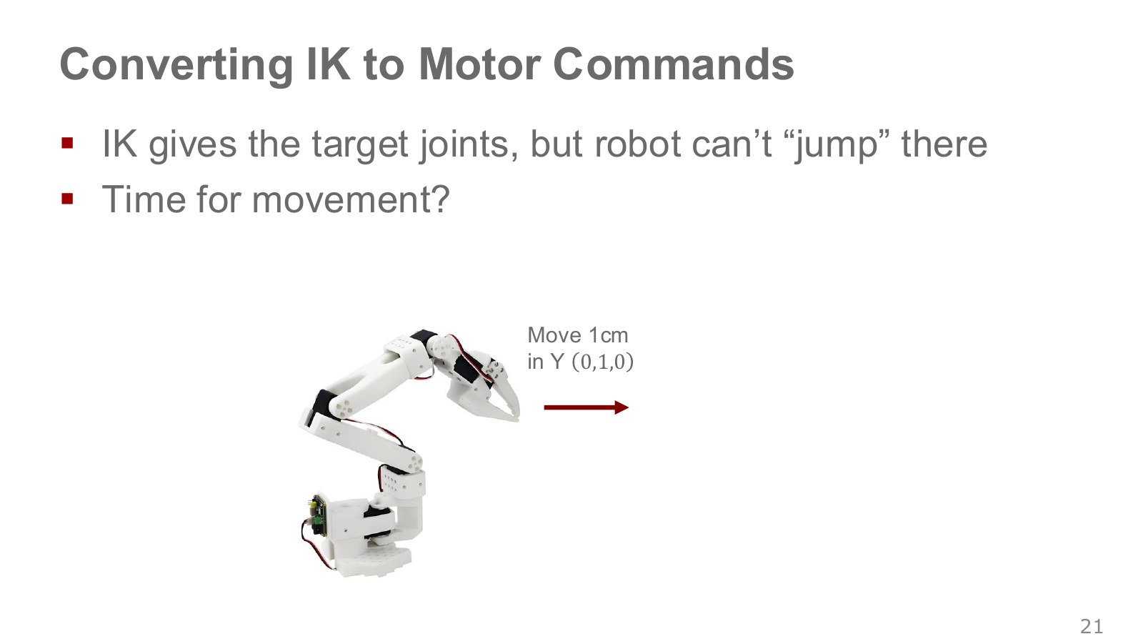
Even when IK supplies target angles, a robot cannot jump instantly from its current pose. We need a sequence and timing for the joints between the endpoints, then drive them while monitoring measurements. This is the step from specifying a target pose to executing a movement.
Even “1 cm along ” needs a specified frame. The tool-frame axis can differ from the base-frame axis. For straight-line hand motion, we can first define a path in task space and solve IK along it. Linear interpolation between starting and ending joint angles generally does not produce a straight tool-tip path.
#P023 · Linear interpolation: generating intermediate targets over time
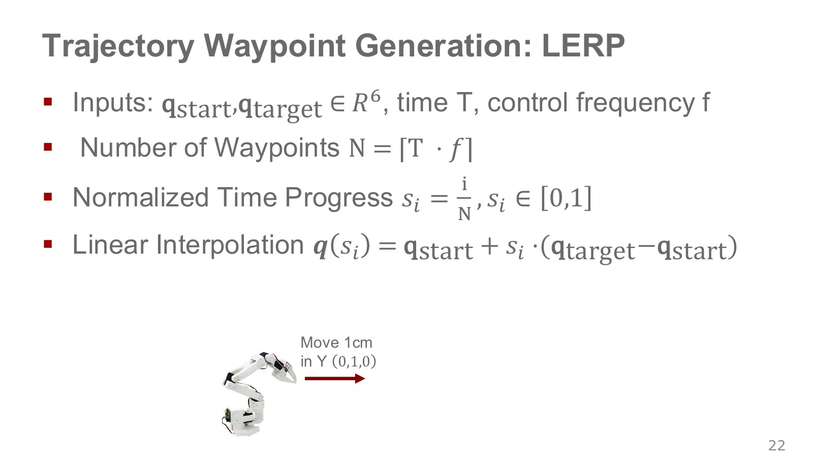
For a move lasting seconds at control frequency Hz, the time interval is approximately seconds. As an illustrative convention, define as the number of intervals and generate points including both endpoints. Under that convention, the slide’s interpolation is:
Explore the symbols and calculation Linear interpolation generates intermediate joint targets from normalized progress between starting and target configurations
Read the equation in words
Divide the change from start to target by uniform progress to generate intermediate joint targets. Linear joint changes need not produce a straight tool-tip path in space.
Understand each symbol
- The configuration vector collecting all joint positions. Revolute joints normally use radians and prismatic joints use length units.
- Progress at point . Here counts interpolation intervals, not data samples.
- The initial and final joint configurations.
Follow the calculation
- Use interval count and the current interval index to compute progress from 0 to 1.
- Multiply the complete joint change by progress and add it to the starting value.
Check with a small example
Four intervals from 0 rad to 1 rad give targets 0, 0.25, 0.5, 0.75 and 1 rad.
An illustrative example for understanding the equation.
is progress from 0 to 1. Moving one joint from 0 rad to 1 rad in one second with gives and 101 points including both endpoints. The first target is 0, the middle target 0.5 and the last 1 rad. If an implementation adjusts timing through rounding, the actual must also be specified.
A robot’s need not be six-dimensional as in the slide example. Use a vector matching its joint count and account for limits and angle boundaries. This step generates a target trajectory; it is not a measurement showing that the motors followed it.
The instruction to move the hand 1 cm becomes tool-tip target → IK joint target → intermediate joint targets over time. Example, 22:22–23:54. Denser intermediate targets do not remove the need to align observations and targets in time. If a 100 Hz controller follows goals from a 10 Hz policy, specify which target it uses for the ten control updates between policy calls. It may hold the target or interpolate according to time.
Intermediate targets are called waypoints. Linear interpolation is also abbreviated LERP. It moves a fraction of the way from start to end: progress 0 gives the start, 1/2 gives the midpoint and 1 gives the end. Control frequency determines how often such targets are updated; it is not itself the motor’s physical speed.
#P024 · Continuous position can still have abrupt velocity changes
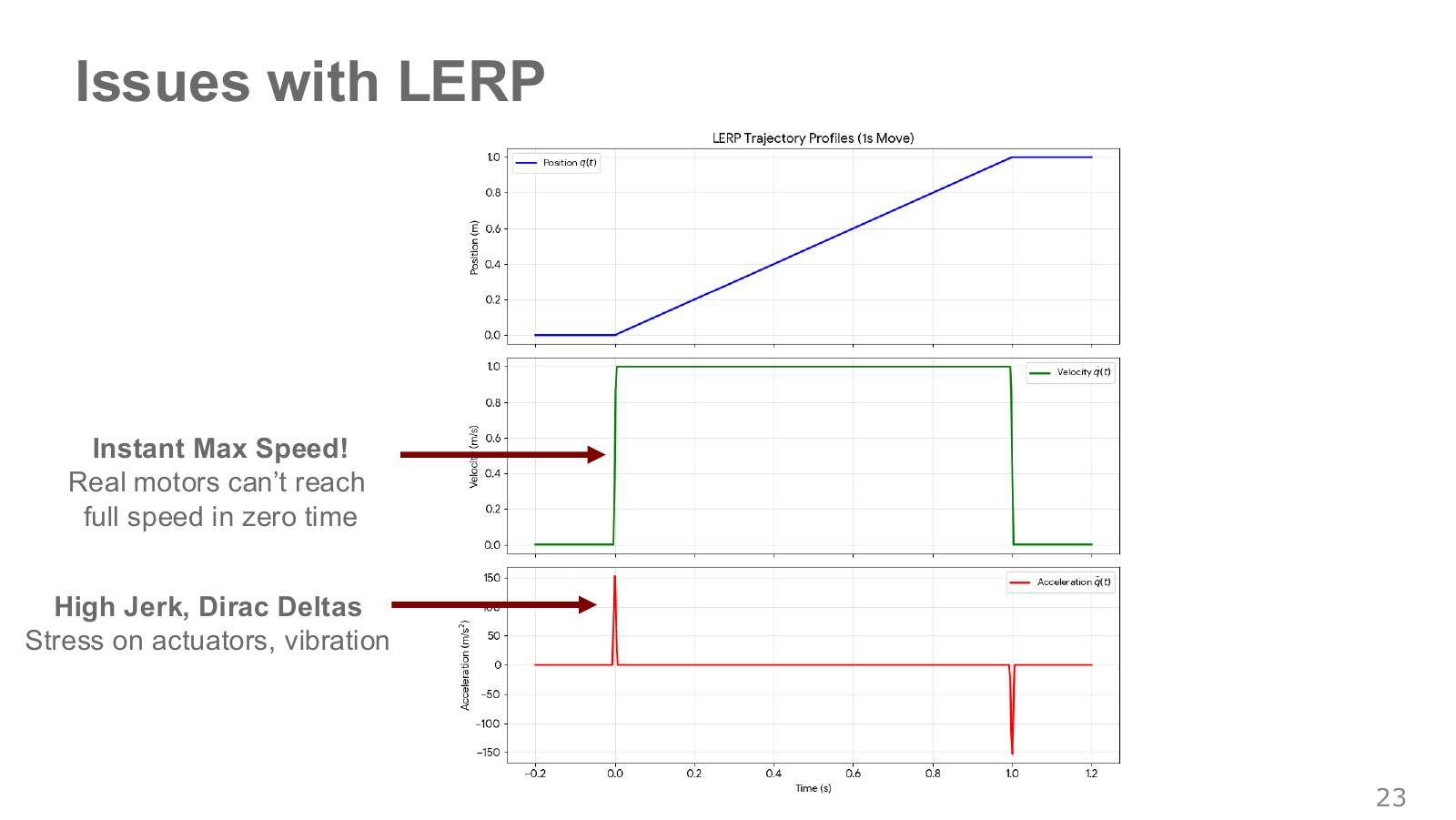
Linear position interpolation gives constant velocity during the move. Before the move the robot is stationary, then instantly switches to that velocity, and stops again at the end. In idealized continuous time, those velocity jumps require impulsive acceleration. Real motors cannot follow them exactly and may develop tracking error or vibration.
Read the three graphs from top to bottom. The blue position line runs straight from the start at 0 seconds to the target at 1 second. Its constant slope during movement gives the constant green velocity line in the middle. The problem lies at departure and arrival: velocity jumps from zero to the moving value and drops straight back to zero at the target. An unbroken position curve alone does not make a command smooth.
Changing velocity requires acceleration. The same velocity change requires greater acceleration when made over less time; in the ideal limit of zero change time, no finite acceleration value represents it. The red spikes at the bottom mark the impulsive accelerations at start and stop. Their finite drawn heights should not be read as a motor’s maximum acceleration. They indicate that the command itself requires instantaneous changes in velocity.
A time derivative measures how quickly a quantity changes over time. Differentiating position once gives velocity and twice gives acceleration; the rate of change of acceleration is jerk. One dot denotes one time derivative, and two dots denote two.
Explore the symbols and calculation Successive time derivatives of position give velocity, acceleration and jerk
Read the equation in words
Velocity is how quickly joint position changes with time; acceleration is how quickly velocity changes. Jerk is the rate of change of acceleration.
Understand each symbol
- The configuration vector collecting all joint positions. Revolute joints normally use radians and prismatic joints use length units.
- First, second and third derivatives with respect to time.
- Here this is continuous physical time.
Follow the calculation
- Differentiate position once with respect to time to obtain velocity.
- Differentiate again for acceleration, then again for jerk. The number of dots gives the derivative order.
Check with a small example
For , velocity is , acceleration , and jerk 6. With position in rad, their units are rad/s, rad/s² and rad/s³.
An illustrative example for understanding the equation.
If position is expressed as as in this figure, the successive units are m/s, m/s² and m/s³. For joint angles in radians, they are rad/s, rad/s² and rad/s³. Abrupt acceleration and braking can require large forces or torques and excite vibration. The next step therefore goes beyond adding intermediate positions to create a schedule that gradually accelerates from rest and slows before the target. Video, 23:58–24:48.
#P025 · Quintic time scaling for smooth starts and stops
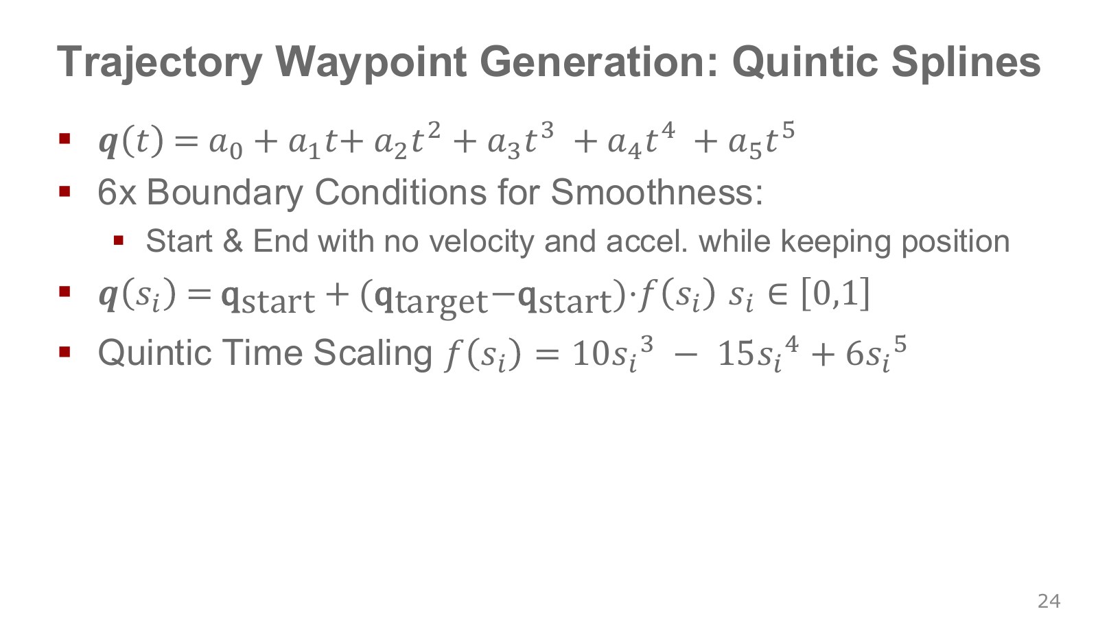
Two position conditions, two zero-velocity conditions and two zero-acceleration conditions give six boundary conditions. A fifth-degree polynomial with six coefficients can satisfy them. To distinguish it from other functions, write the slide’s expression in normalized time as .
Explore the symbols and calculation Quintic time scaling satisfies endpoint positions and zero velocity and acceleration at both ends
Read the equation in words
Shape motion progress so that endpoint velocity and acceleration are zero. This reduces the abrupt start and stop of linear interpolation.
Understand each symbol
- The fraction of total time elapsed, ranging from 0 to 1.
- A fifth-degree function that smoothly varies progress.
- Starting joint values, target joint values and total duration. The subscripts distinguish the endpoints here.
Follow the calculation
- Divide current time by total duration to obtain normalized progress.
- Transform progress through the quintic polynomial and multiply it by the total joint displacement.
Check with a small example
For start 0 rad and target 1 rad, normalized time 0.5 also gives polynomial progress 0.5. Endpoint velocity and acceleration are zero, but jerk need not be zero.
An illustrative example for understanding the equation.
are the start and end joint vectors. and , with equal to zero at both endpoints. The joint-space path stays the same while its progress over time changes: the motion starts slowly, speeds up in the middle and gradually stops.
The Modern Robotics trajectory video and script (video, 1:19–2:49) compares cubic, quintic, trapezoidal and -curve time scaling. Satisfying the quintic boundary conditions does not automatically satisfy every actuator’s velocity and acceleration limits.
The six conditions specify starting and ending positions, velocities and accelerations. They determine both the endpoints and how the motion joins the stationary periods before and after it. Choosing the six quintic coefficients accordingly makes position, velocity and acceleration continuous into those stationary periods. The conditions do not require jerk to join them at zero.
#P026 · Even a smooth trajectory needs enough time
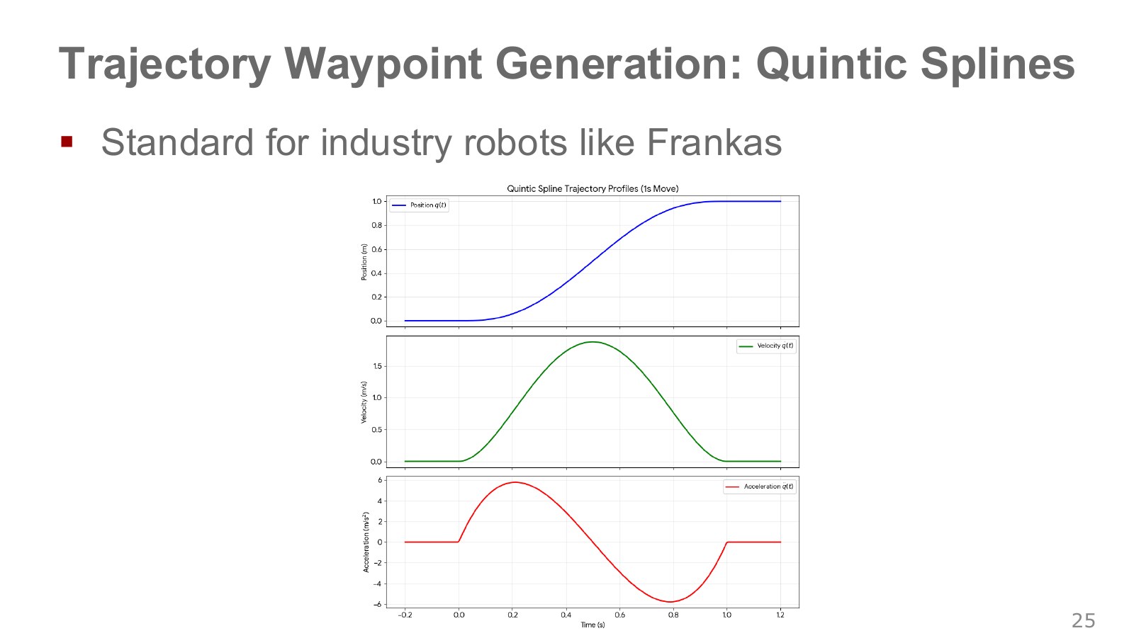
Differentiating with respect to time shows that velocity scales with and acceleration with . Completing the same move in half the time doubles peak velocity and quadruples peak acceleration. A smooth expression and a motion the motors can sustain are different requirements.
For a joint moving from 0 rad to 1 rad in one second, this quintic has a peak velocity of 1.875 rad/s, exceeding the 1 rad/s linear-interpolation speed over the same interval. It travels faster in the middle to allow gentler starts and stops. The figure below was computed directly from the expression.
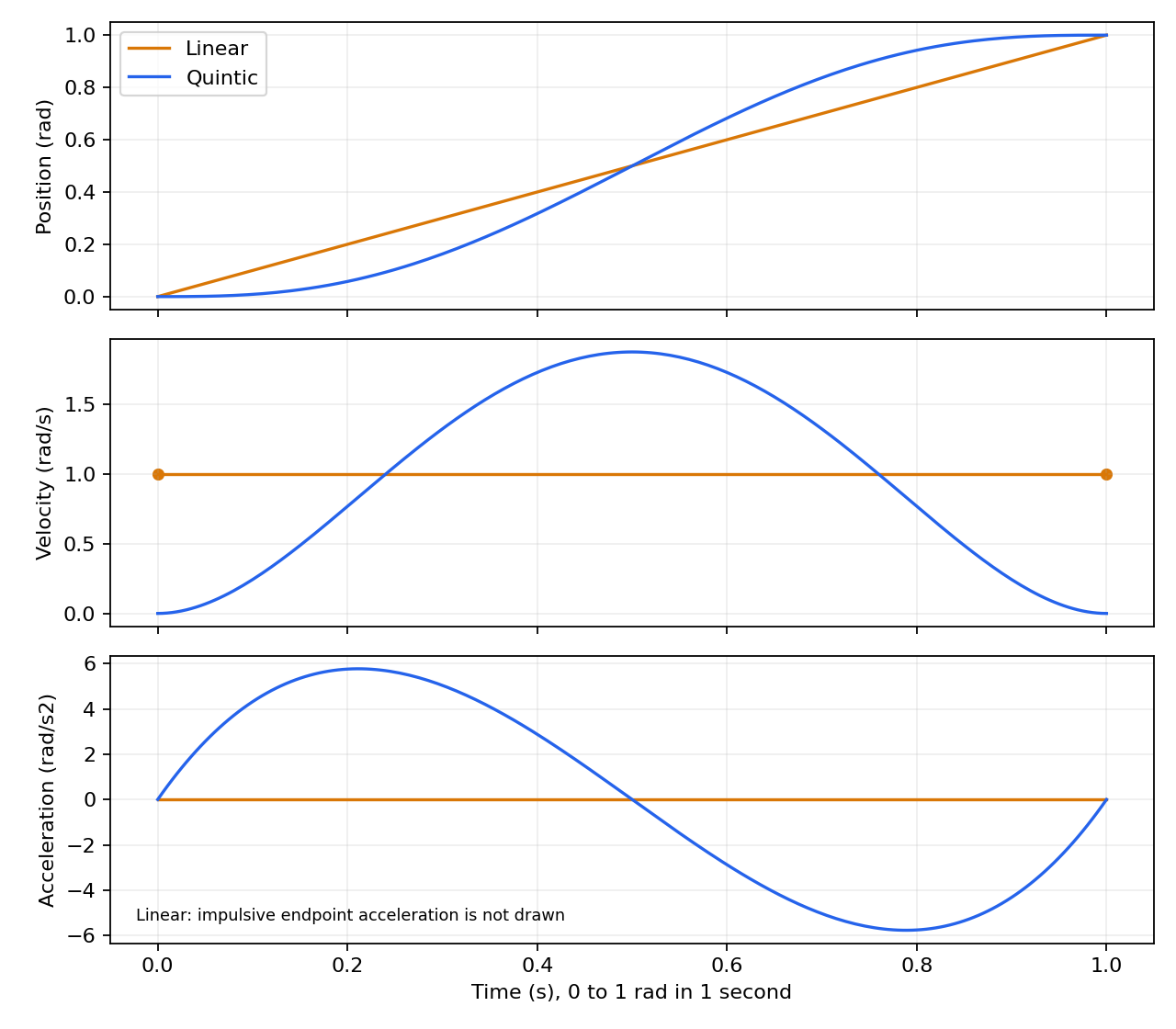
Use joint velocity and acceleration limits to increase or select another time scaling. Continuous position, velocity and acceleration do not imply continuous jerk; choose according to the required motion quality.
For the 1 rad move above, a maximum allowed velocity of 1 rad/s requires at least 1.875 seconds under this quintic, considering velocity alone. Acceleration or torque limits can require longer. As Modern Robotics, 2:40–2:49 emphasizes, motion speed depends on distance and total duration as well as curve shape.
When comparing LERP with a quintic along the same path, hold displacement and duration constant. Storing more samples does not by itself mean the robot moved more slowly or smoothly.
This velocity graph has a rounded peak instead of a rectangle. Velocity rises gradually from zero, peaks near the middle and decreases before arrival. Acceleration is positive early and negative later. The later negative acceleration means braking to reduce forward speed, not moving backward. Reading its sign alongside the position graph explains how the same goal can be reached with less abrupt motion.
#P027 · PID: correcting the difference between a planned trajectory and measurements
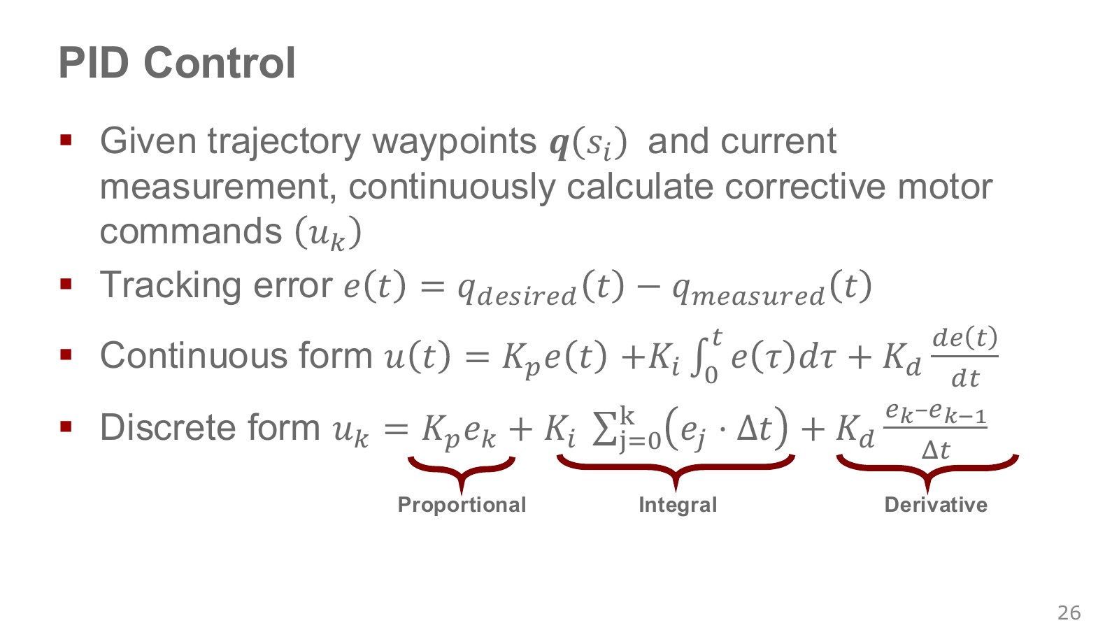
Gravity, friction and payload make real joints depart from their target trajectory. PID control repeatedly reads the difference between target and measurement and computes a corrective command. Here error is target minus measured value.
Explore the symbols and calculation Discrete PID combines current error, accumulated error and error rate to form an actuator command
Read the equation in words
Combine target-minus-measurement error, its accumulation and its rate of change into a motor command. This is feedback between the desired trajectory and actual motion.
Understand each symbol
- Target minus measured value. Its sign convention differs from the position-IK error above.
- The command sent to the actuator, measured in torque for torque control.
- Gains multiplying current, accumulated and rate-of-change errors.
- The actual time interval between successive measurements.
- Add every term over the indicated range, computing one term and repeating through the end of the range.
Follow the calculation
- Subtract measured position from target to obtain current error.
- Compute and add the proportional term, the time-accumulated term and the term using the difference from the previous error.
Check with a small example
Current error 0.2, previous error 0.1 and interval 0.1 seconds give error rate 1. With proportional gain 10 and derivative gain 2 only, the command is .
An illustrative example for understanding the equation.
are the three gains and is the measurement/command interval. The proportional () term reacts to current error, the integral () term to accumulated error, and the derivative () term to how quickly error changes. Gain units depend on whether the input error and output command represent angle, velocity or torque.
For a numerical example, take current error 0.1, previous error 0.12, and accumulated integral 0.2. With , the three terms are , and , giving a command of −0.9. Even while the joint remains short of its goal, the derivative term can brake if it is approaching quickly. These values illustrate a calculation, not recommended gains for a real robot.
The integral adds the area of error accumulated over time. In a computer, multiplying each sampled error by the time interval and adding turns it into a sum. The derivative is likewise approximated by the change from the previous error divided by the interval. The term uses the current shortfall, tracks persistent lag, and tracks rapid approach. Sending the computed command, taking a new measurement and repeating the process closes the feedback loop.
#P028 · Reading PID as a spring, accumulated correction and a damper
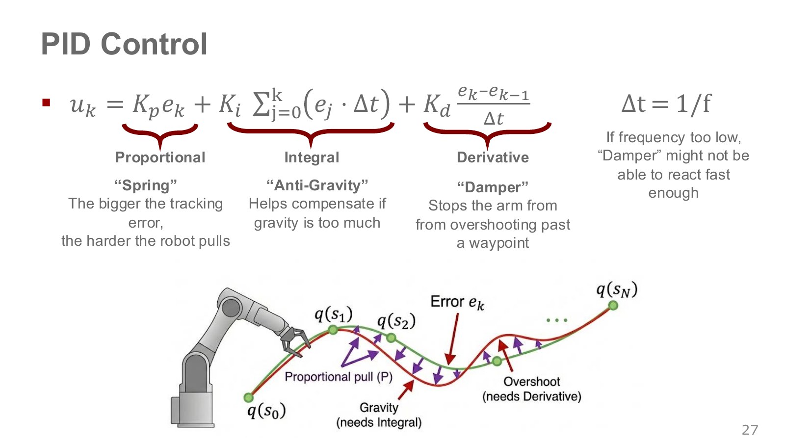
A spring pulling harder as displacement from the target grows provides an intuition for . The term accumulates persistent error to add correction, while reacts to rapid error changes and can reduce an excessive approach. Hence the analogies of as a spring and as a damper. PID analogies, 25:55–27:51. The integral term does not directly identify gravity; it accumulates sustained error, unlike gravity compensation based on a dynamics model.
Arbitrarily increasing gains can cause oscillation or actuator saturation. The integral term needs protection against windup while commands saturate, and the derivative can amplify sensor noise. Changing control frequency changes , so the behavior of the same numerical gains needs checking again.
A common arrangement has a policy choose target joint positions relatively slowly and a lower-level controller track them faster. The official ETH assignment below also separates policy calls from physics steps.
For a more concrete view of the integral term, Modern Robotics on torque control, 0:09–1:36 considers a single joint tracking a fixed target under gravity. If a PD controller holds the joint stationary against gravity torque , the derivative term is zero and the following equilibrium is required.
Explore the symbols and calculation At a stationary PD equilibrium without gravity compensation, proportional torque may require nonzero steady-state error
Read the equation in words
If proportional control alone must supply torque against gravity, an error between target and measured position can remain even at rest.
Understand each symbol
- The steady-state error remaining after the motion settles.
- The torque needed to support against gravity.
- The proportional gain converting position error into torque.
Follow the calculation
- At rest, the derivative term is zero.
- Divide the torque needed against gravity by the proportional gain to calculate the residual position error.
Check with a small example
Gravity torque 2 Nm and proportional gain 10 Nm/rad leave error rad. Gravity compensation or an integral term changes this equilibrium relationship.
An illustrative example for understanding the equation.
is the steady-state error remaining after sufficient time. With required torque 1 N· at the given configuration and , the example needs 0.05 rad of error for the proportional term to supply that torque. An integral term retains accumulated past error and can therefore produce torque even when current error reaches zero. This account assumes a stable, unsaturated equilibrium at a fixed target; it does not model every robot’s gravity effects with one constant.
At 4:32–5:10 in the same video, adding an integral term reduces steady-state error but introduces overshoot. Another approach is to add the required torque in advance using a gravity model. Connecting PID to actual motion requires considering error reduction and stable operation together.
The green markers on the path are target waypoints. If the arm sags below its target, pulls in a direction reducing the error. Persistent sag under gravity accumulates in , adding correction. Approaching too fast and passing the goal is overshoot, and can brake that change. When the target itself moves, however, its velocity also affects ; describing it as “always a brake” does not explain every PID behavior.
#P030 · From knowing how to move to choosing the next action
So far we have asked how to move toward a specified target. We still need to choose the next target: whether to move an obstacle before grasping a cup, or approach again after missing an object.
A learned policy can output a tool-tip goal executed through IK, trajectory generation and a lower-level controller. Other systems output joint positions or torques directly. Which layers the policy handles changes both the meaning of its actions and the difficulty of learning them.
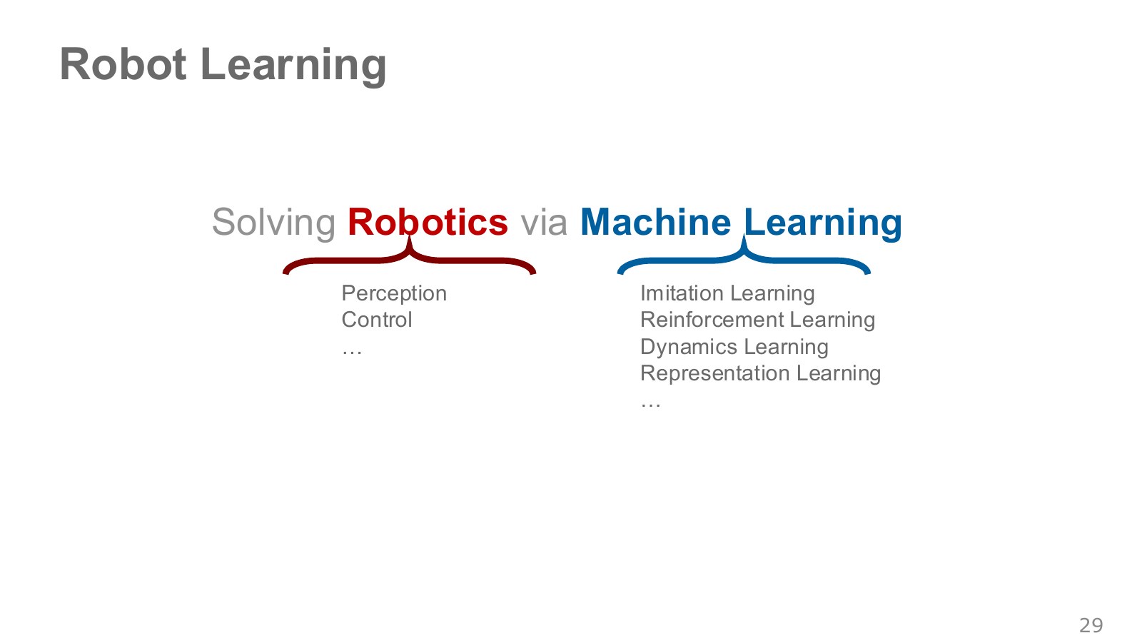
Machine learning can also enter at several points. Perception estimates cup and hand locations from images; imitation learning teaches a policy the observation–action relationships demonstrated by a person. Reinforcement learning improves choices using execution rewards, dynamics learning predicts state changes after actions, and representation learning extracts task-relevant features from sensor values or images. These modules can be combined; they need not form one model that directly outputs motor commands.
Even with a good trajectory-tracking controller, we still need to choose which trajectory to follow. If the cup moves or a new obstacle appears, the system must decide which object to grasp first and how to sequence its movements. After learning how to execute a specified motion, we now turn to the rule that chooses the next motion from observations. From control to decision-making, 27:54–29:00.
#P031 · A sequence of actions makes one task
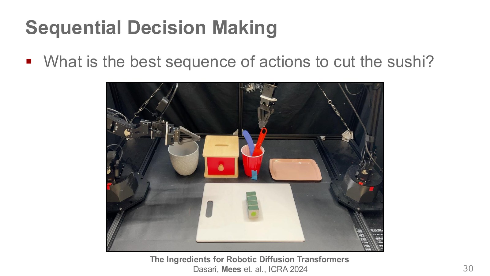
To cut toy sushi with a two-arm robot, one hand first grasps a tool and moves it so the other can take it, then the tool must be aligned with the object and moved appropriately. Even with toy food, precision and sequencing are needed to fit small gaps. Two-arm task video, 29:02–30:38. The central issue is choosing the current action to make the next stage possible, rather than producing one impressive pose.
In the ALOHA demonstration, one hand picks up and passes the knife; the other receives it and cuts the toy sushi. An error in the earlier stage can prevent the receiving hand from taking the knife, so the full sequence matters. The policy generates successive commands at high frequency, while the lower-level controller corrects motor-tracking errors.
Even a small position error in the hand holding the knife is not enough to describe success: grasping in the wrong sequence can make later steps impossible. Each action changes the next observation and which actions become possible. This is a sequential decision-making problem.
For instance, the tool must be held stably before cutting, and the other hand may need to secure the object to prevent slipping. Creating the contact needed for the next step can be more useful than immediately moving closer to the target. Evaluation therefore expands from instantaneous pose accuracy to actions and consequences over the whole task.
The lecture describes this two-arm example as having 14 degrees of freedom. The task requires continuously updating both arms’ drives to preserve the tool–object relationship, rather than matching one hand position. The horizon describes how far ahead these decisions are considered. Over a long horizon, a small choice now can change the chance of success many steps later. A higher-level policy makes these choices, while lower-level controllers such as PID track the goals through actual joint motion. Two arms and control layers, 29:02–30:38.
#P032 · What classification and policy networks share—and where they differ
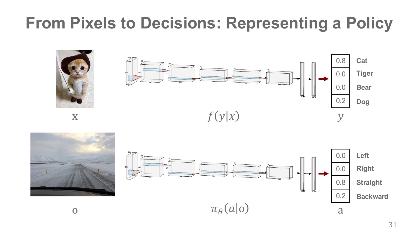
A cat-image classifier computes class scores or probabilities from an image. A policy network can similarly compute action probabilities, such as left or right, from a camera image. The 0.8 in the figure is the probability of selecting that output for the current input, not a success rate or reward.
The key difference emerges after using the output. Misclassifying a photograph does not change the cat in it, but steering a car incorrectly changes the next camera image. Predicting one target in a labeled dataset and repeatedly acting in a real closed loop therefore require different evaluation.
NTU’s RL introduction, 5:00–6:28 calls this observation-to-action function an Actor. Finding the function involves more than predicting the answer for one input. It means using the function to act in the environment, receive changed observations and improve the sum of rewards over multiple steps. ETH’s , NTU’s Actor and the observation-to-torque function in the exercise below connect through this input/output view. A fixed PD function sharing the interface is nevertheless not a policy learned from rewards.
The output bars give forward and reverse weights of 0.8 and 0.2, with left and right at zero. Interpreted as discrete probabilities, they sum to 1. Choosing the largest gives forward; sampling can also select reverse. A high learned probability does not guarantee safety or success. Evaluation must include the input sensors and the scene changed by execution.
#P033 · Policies receiving states and policies receiving observations
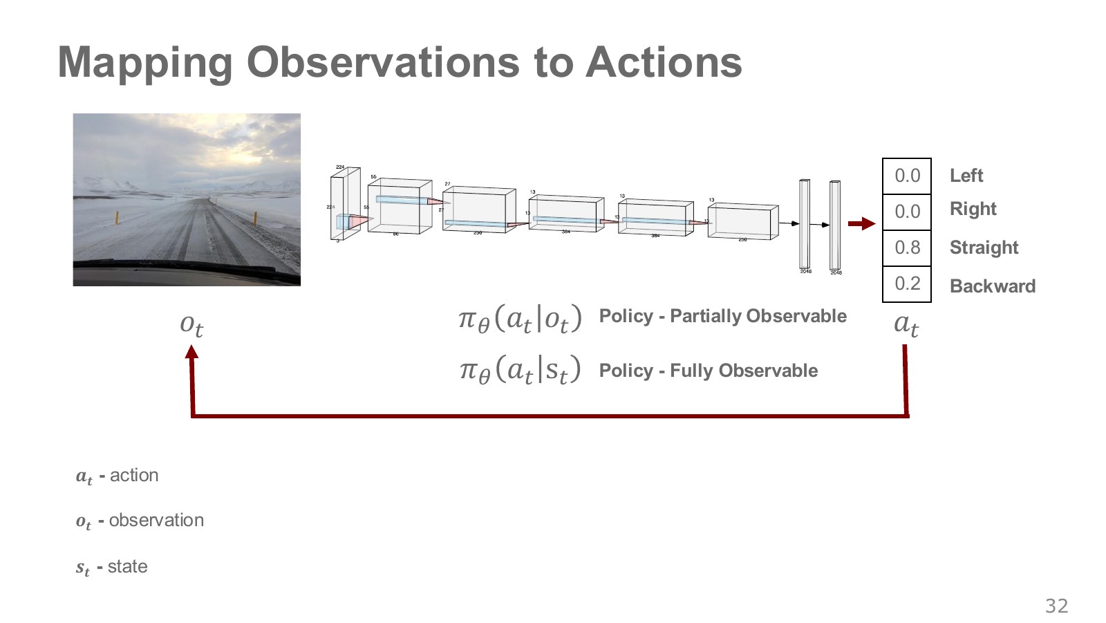
At time step , write the state as , observation as and action as . A stochastic policy defined by network weights can be written as follows.
Explore the symbols and calculation A policy forms an action distribution conditioned on the current observation or accessible state
Read the equation in words
The expression distinguishes a policy receiving observations from one receiving state directly. Those inputs need not contain the same information.
Understand each symbol
- The action chosen at step : for example, a torque, a joint target or a movement direction, depending on the setup.
- The sensor observation at step . It is not assumed to equal the full physical state.
- The state at step , containing information such as position and velocity needed to predict what happens next.
- A policy choosing actions given a state. A stochastic policy outputs probabilities or probability densities for actions.
- The parameters collecting the trainable weights of the network or policy.
- Conditional notation: the information to the right of the bar is given. This is not a division sign.
Follow the calculation
- First specify the information actually accessible to the policy.
- Compute the corresponding action distribution and choose an action.
Check with a small example
A policy receiving one photograph may not know object velocity. Its input conditions differ from those of a policy receiving both position and velocity.
An illustrative example for understanding the equation.
The bar means “given this information,” and means “sample from the distribution.” For continuous actions, the output can be a distribution over torques or position changes rather than probabilities for buttons. A deterministic policy produces one action for a given input.
Using only one observation is a simple policy choice under partial observability. Policies may instead use a history of images and actions or internal memory. Merely renaming the current observation does not supply missing information.
The red downward arrow traces the output action through the environment and back to the next image. A network diagram may look like a single input-to-output calculation, but a robot repeats it over time. Subscript indexes the step in that repetition; policy subscript denotes the learned weights instead. Distinguishing them separates information arriving over time from the rule that uses it to choose actions.
Time subscripts 0, 1 and 2 in these notes are decision-step indices, not seconds. At 10 Hz, a policy step lasts 0.1 seconds; at 100 Hz it lasts 0.01 seconds. Three steps can therefore cover different amounts of physical time. Keep this convention when reading trajectory probabilities and discount factors below.
#P034 · The same physical situation can look different
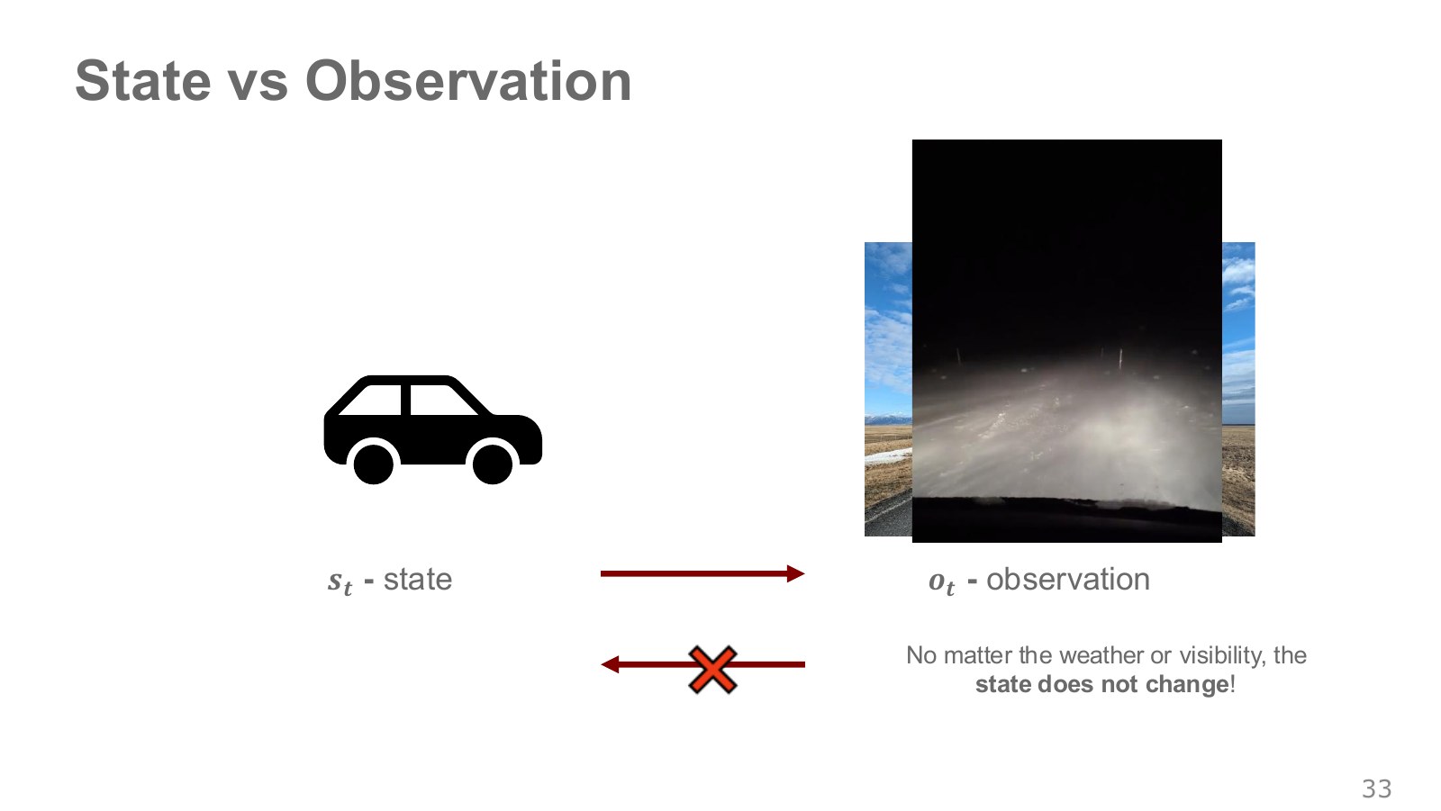
Let a car’s state include position, velocity and heading, and let its observation be a camera image. Lighting or fog can change the image greatly at the same position and speed. Conversely, similar images can occur at different speeds or with different occluded obstacles. In general, observations do not guarantee exact recovery of state.
The slide’s statement that state is unchanged by weather should be read as holding a chosen car-motion state fixed while varying visibility. If weather changes friction or motion, its effects belong in the state, disturbance or transition model. The example does not claim that real weather changes leave every physical state unchanged.
The wall-facing camera robot in DeepMind/UCL Lecture 1, 43:52–45:17 raises the same issue. Having looked behind a moment ago may matter for the next action. The relevant extension is a partially observable MDP (POMDP).
The next illustration is the original diagram from page 38 of the UCL Lecture 1 PDF. Observing only nearby cells, rather than the whole map, can make two locations indistinguishable.

The video at 47:31–51:08 asks the agent to move from the upper right to the upper left. The highlighted observations are identical, but the right-hand location requires going down and around, while the left-hand one requires going up. A function receiving only one observation has no basis for different answers. Adding one previous observation is not always enough in this maze either. The point is to include the history needed to distinguish the current situation in the state representation, rather than mechanically increasing frame count.
#P035 · The Markov property does not mean ignoring the past
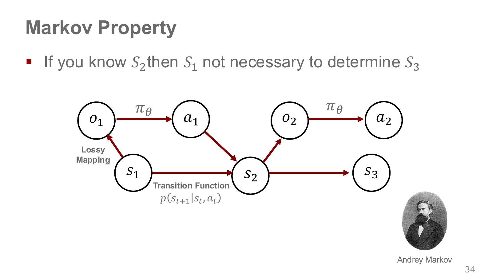
A process has the Markov property if, given the current state and action, adding earlier history does not change the conditional distribution of the next state. For a controlled process, this is:
Explore the symbols and calculation Given current state and action, earlier history adds no information for predicting the next-state distribution
Read the equation in words
The Markov property says current state sufficiently summarizes past information needed for prediction. It does not automatically hold for one current photograph.
Understand each symbol
- The probability of a next state after acting in the current state, or its density for continuous states.
- The state at step , containing information such as position and velocity needed to predict what happens next.
- The action chosen at step : for example, a torque, a joint target or a movement direction, depending on the setup.
- Conditional notation: the information to the right of the bar is given. This is not a division sign.
Follow the calculation
- Fix the current state and action.
- Consider whether adding earlier history changes the conditional next-state distribution.
Check with a small example
At the same position, velocities +1 and −1 produce different next positions. Position alone may be insufficient, while position together with velocity supplies more predictive information.
An illustrative example for understanding the equation.
For example, identical joint angles alone can lead to different next positions when velocities differ. Angles alone may therefore be an insufficient state for this model. Joint velocities and relevant object states may also be needed. The condition says that the required information is compressed into the current state; it is not an instruction that discarding past observations is always correct.
A Markov transition can still be stochastic. ETH, 34:52–36:00 · UCL, 40:49–43:17. Having sufficient current information and having one determined future outcome are different claims.
Controller memory can be understood in the same way. Even with identical current joint angles and velocities, different accumulated integral values make a PID controller issue different commands. Modeling PID as a memoryless function of current joint measurements misses that distinction. To predict the system including its controller, consider whether the integral accumulator and required previous errors belong in the state.
A “sufficient state” need not literally copy the whole world; it is a choice of information suited to the system and time interval we want to predict. Applying the state–action diagram from ETH, 34:52–36:00 to real control code leads to this question.
The “lossy mapping” arrow from state to observation indicates that sensing may lose information. One photograph need not reveal actual vehicle speed or an occluded object’s position. The state-and-action-to-next-state arrow instead describes environmental changes through motion, contact and other processes. Distinguishing the arrows separates a need for more sensor information from a need to better predict physical action outcomes.
#P036 · Recognizing alternative notation for state, action and cost
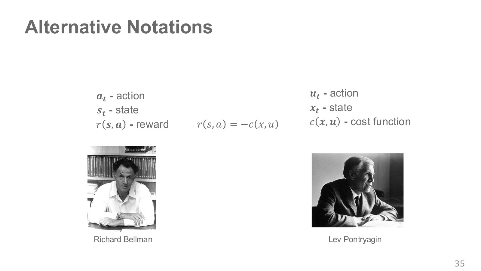
Robot-control literature often writes state as , input as and cost as . Reinforcement-learning literature often uses , and for state, action and reward. Match the physical quantities and time steps rather than relying on symbol names.
Under matching conditions, setting makes minimizing cumulative cost express the same preferences as maximizing cumulative reward. The horizon, discounting and termination conditions must match too. Hand position in inverse kinematics and full state here may use the same letter for different roles.
#P037 · An MDP combines states, actions, transitions and rewards
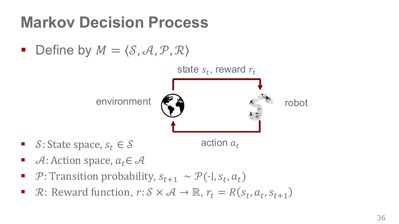
An MDP makes the ingredients of a decision problem mathematically explicit. Its four basic elements are states, actions, transitions and rewards. An actual learning problem also specifies the initial-state distribution and a horizon or discounting conditions.
| Element | Meaning | What to specify for cup grasping |
|---|---|---|
| State space | The set of possible states | Which joint angles, velocities, cup positions and contacts are included? |
| Action space | The set of possible commands | Tool-tip targets, joint targets or torques? |
| Transition | How a state and action produce a next state | How do gravity, friction, contact and lower-level control act? |
| Reward | A numerical rule evaluating action outcomes | How are grasp success, elapsed time and collisions reflected? |
The slides use both and for rewards. Here, we define the reward from moving from to under action as , and write the interaction as follows.
Explore the symbols and calculation After an action, obtain the next state from the transition distribution and compute that transition's reward
Read the equation in words
Executing an action lets the environment produce the next state and a reward for that transition. This creates one transition record for learning.
Understand each symbol
- The state at step , containing information such as position and velocity needed to predict what happens next.
- The action chosen at step : for example, a torque, a joint target or a movement direction, depending on the setup.
- The probability of a next state after acting in the current state, or its density for continuous states.
- The reward received at one step: a learning signal defined so that larger is better.
- The function assigning a numerical reward to a transition outcome. Uppercase names the reward function here.
- Conditional notation: the information to the right of the bar is given. This is not a division sign.
Follow the calculation
- Obtain the next state from the transition distribution for the current state and action.
- Pass the current state, action and next state into the reward function.
Check with a small example
A grasp action that moves from a pre-lift state to a state with the cup lifted could receive success reward 1 for that transition.
An illustrative example for understanding the equation.
Another book may call the same transition’s reward . Align the indexing convention before calculating. A more general model can also make rewards stochastic. Defining an MDP does not mean a good policy has already been found. The learning algorithm determines which experiences to collect and how to improve the policy within that framework.
David Silver’s student Markov chain in Lecture 2 is useful practice for reading states and transitions.
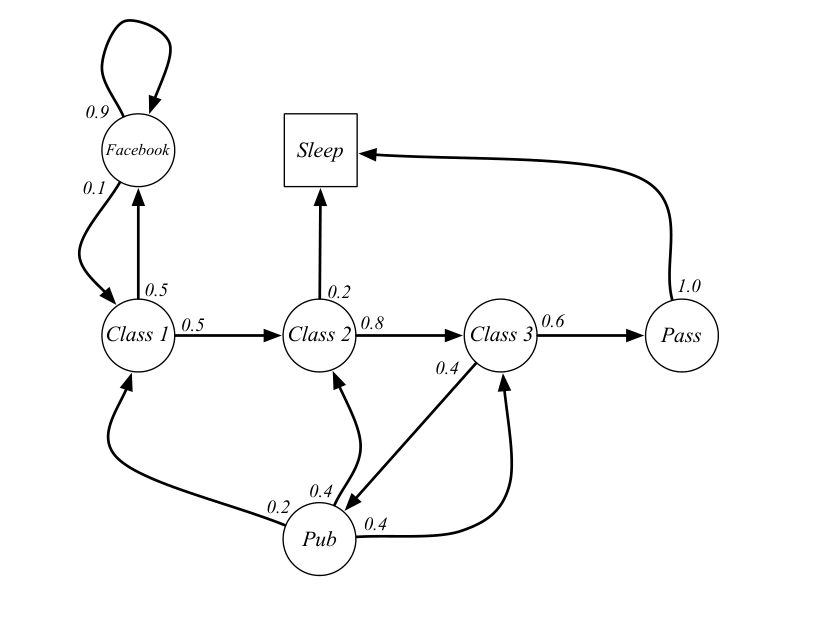
The two arrows leaving Class 2 give probability 0.8 of moving to Class 3 and 0.2 of moving to Sleep. Next-state probabilities from one state sum to 1, and this diagram has no action choice yet. Chain explanation, 7:28–8:55. Adding actions such as Study and Sleep, each with different transition probabilities, extends it into an MDP. Example with actions, 43:37–46:24. What the agent chooses changes the next-state distribution.
Once the policy is fixed, we can calculate the transition it induces. For discrete actions, the following expression averages action-specific transitions using the policy’s action probabilities.
Explore the symbols and calculation Under a fixed policy, state transitions average action-specific transitions by their selection probabilities
Read the equation in words
Fixing a policy incorporates action selection into the average state transition. Sum action-specific outcomes weighted by the policy's selection probabilities.
Understand each symbol
- A policy choosing actions given a state. A stochastic policy outputs probabilities or probability densities for actions.
- The probability of a next state after acting in the current state, or its density for continuous states.
- The state-transition distribution after averaging over the policy's action choices.
- Add every term over the indicated range, computing one term and repeating through the end of the range.
- Conditional notation: the information to the right of the bar is given. This is not a division sign.
Follow the calculation
- For each action, obtain the probability of reaching the same next state.
- Multiply each by that action's selection probability and add.
Check with a small example
Choosing left with probability 0.7 and right with 0.3, with respective success probabilities 0.8 and 0.4, gives average success probability .
An illustrative example for understanding the equation.
As a separate example, suppose that from state a left action reaches / with probabilities 0.8/0.2, while right reaches / with probabilities 0.1/0.9. If the policy chooses left with probability 0.75 and right with 0.25, the probability of next state is , while has probability 0.375. This illustrates separating and then combining the policy’s random choice with the environment’s random outcome.
Read the interaction loop in order: the robot receives available information and chooses an action through its policy. The environment executes it, produces the next state and returns a reward for the outcome. At the next step, the robot acts again from the new state. Reward is a number assessing an outcome that has already occurred against the objective, rather than an answer command specifying what to do next. The learning algorithm uses these records to improve later choices.
Chess and robots have entirely different bodies and commands, yet both fit the MDP structure of observing a state, acting and evaluating the outcome. This shared form supports applying algorithms across environments. Each environment still needs its own state and action dimensions, transitions and rewards; it does not mean transferring a chess policy directly into a robot. The common MDP framework, 36:52–37:43.
#P038 · Continuous state spaces cannot be stored as exhaustive tables
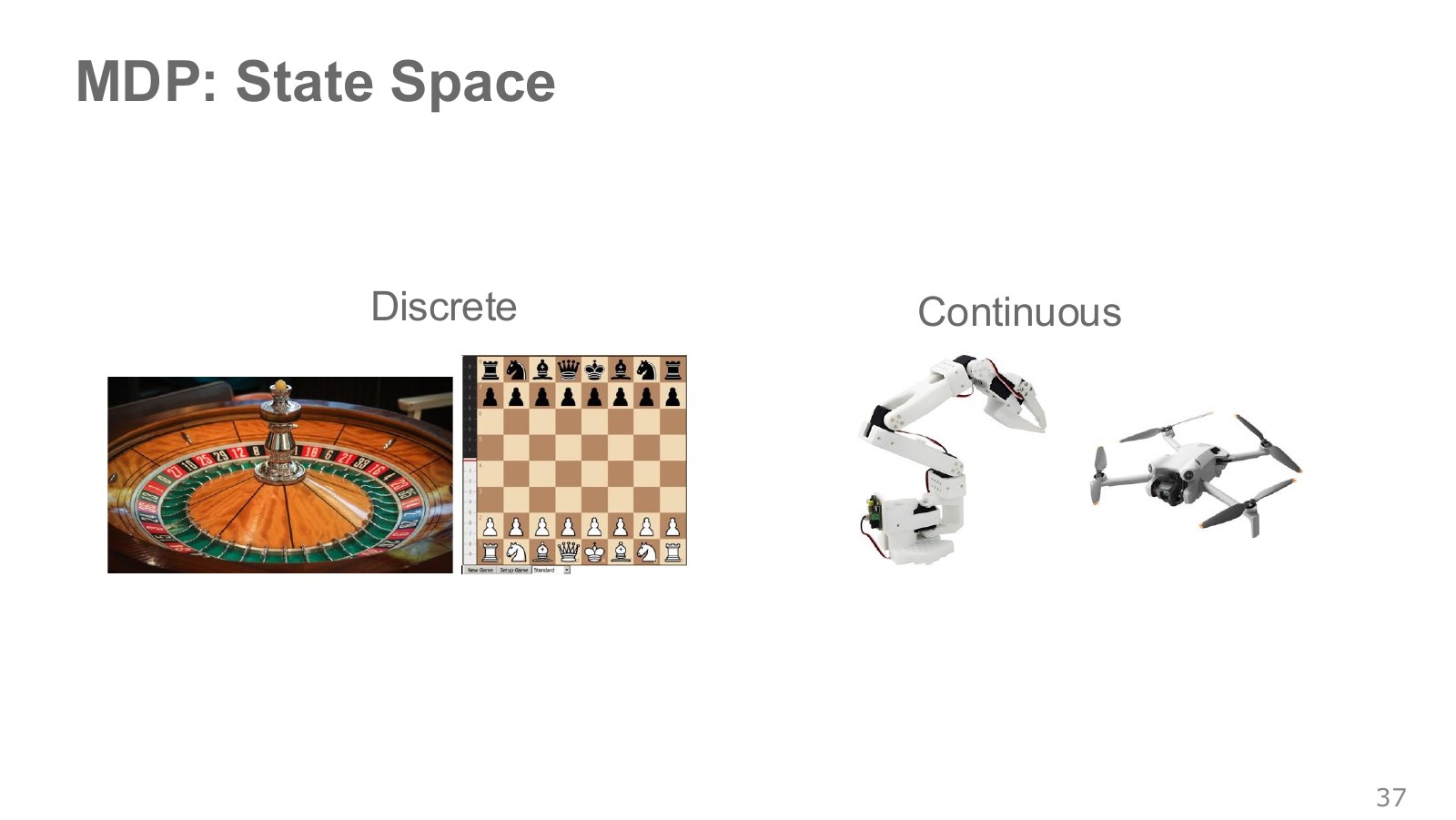
Grid cells and board games can be represented by discrete cases. Joint angles, velocities and object positions are often modeled as continuous quantities. Storing sensor numbers at finite precision is compatible with treating a problem as continuous.
Even dividing each joint angle into just 100 bins gives combinations for seven joints. Adding velocities and object states makes the table grow rapidly. Function approximators such as neural networks share representations and computations across inputs. Applying one to a continuous space does not automatically ensure good behavior in unvisited states.
Even a chess state may need more than visible piece positions. It must include whose turn it is and rule information affecting legal moves. Likewise, a drone at the same photographed position can move differently next if its linear or angular velocity differs. Recognizing objects in a picture and constructing a state sufficient to predict the next outcome are separate tasks.
#P039 · Action numbers need units and execution timing
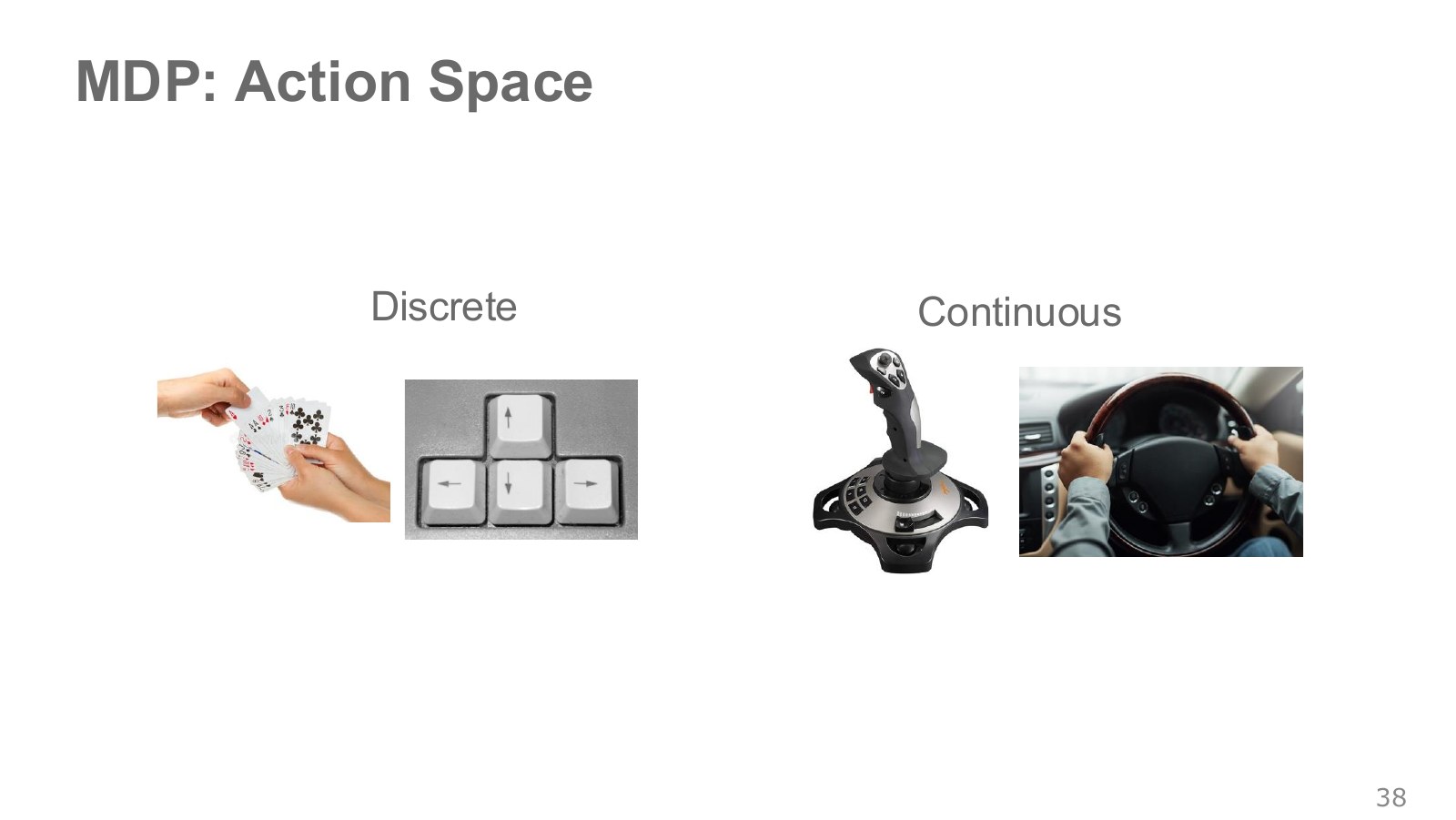
Choosing left or right is a discrete action; selecting a real-valued joint torque is continuous. The same robot can use either depending on its interface. Reading a policy output requires knowing how the environment interprets it.
Distinguish whether is a 0.5 rad target, a midpoint in a normalized range or a torque of 0.5 N·. Applying the same displacement every 0.01 seconds and every 0.1 seconds also produces different motion. Record policy timing, lower-level control timing and physics intervals to reproduce behavior.
The ETH HW2 action-handler description maps normalized into the joint range. For lower and upper joint limits , the linear mapping is:
Explore the symbols and calculation Map normalized actions -1, 0 and 1 to the joint-range lower limit, midpoint and upper limit
Read the equation in words
Convert a neural network's action between −1 and 1 into an allowed physical joint target. A range conversion is distinct from controller design.
Understand each symbol
- The normalized continuous action.
- The lower and upper allowed joint-target values.
- The physical joint target sent to the controller.
Follow the calculation
- Add 1 to the normalized action and divide by 2 to obtain a fraction between 0 and 1.
- Multiply that fraction by the joint-range width and add the lower endpoint.
Check with a small example
For a 0–2 rad joint range, action −1 gives 0 rad, action 0 gives 1 rad, and action 1 gives 2 rad.
An illustrative example for understanding the equation.
For the example range , actions give targets , respectively. Action 0 here is neither a zero joint angle nor zero torque. Inputs that may exceed the range also need clipping.
The MuJoCo actuator documentation describes a position servo that receives a position target and computes force. For a simple revolute joint with unit gear ratio, a position gain acts on the target-minus-current angle and damping reduces motion. The same numerical data.ctrl therefore means different things under XML motor and position settings. Check the boundary where policy output becomes actuator input.
Action representation can also change with the interface used for human demonstrations on the same robot. A keyboard with left, right and stop buttons records a finite, discrete command space. Continuously reading a VR controller’s position and rotation can record continuous target poses. Physically continuous joint angles and the choices offered to a policy are different matters. Either interface needs conventions for converting its inputs to joint or end-effector targets, including units and limits.
#P040 · Transition uncertainty and sensor uncertainty
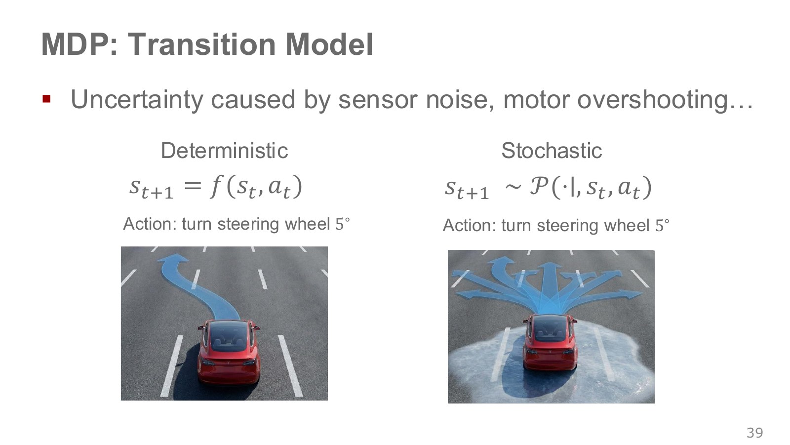
A deterministic model assigns one next state to a given state and action. A stochastic model distributes probability across possible next states. The same steering angle can produce different paths as road friction and actuator errors vary. Steering example, 39:30–40:26.
Make one further distinction: sensor noise creates uncertainty about what was observed, while dynamical disturbances create uncertainty about where the system actually moved. A model separating full physical state from measurements places the former in the observation model and the latter in the transition model. Omitting some factors from state can also make their effects appear as stochastic transitions. Separating them helps diagnose prediction errors versus fluctuating measurements.
The single path on the left models one next outcome for the same state and steering input. The multiple paths on the right assign probabilities to possible outcomes. Stochastic does not mean that everything is equally likely: some directions may be more likely than others. Read it as a modeling choice for uncertainty remaining under a particular state representation and prediction precision, rather than necessarily a claim that the physical world is intrinsically random.
#P041 · Sparse and dense rewards: what counts as doing well?
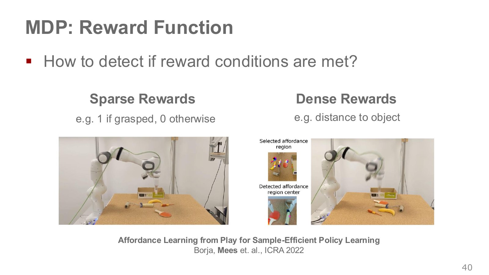
A sparse reward is given infrequently—for example, 1 for a successful grasp and 0 otherwise. Success is clear, but until it happens by chance there may be little signal distinguishing actions. A dense reward also scores intermediate progress, such as the distance between hand and object.
In the lecture’s pick-and-place experiment, rewarding success alone made it difficult to distinguish early failures. A distance reward also signals an approach toward the target. But stopping beside an object and actually picking it up and moving it require a separate final-success criterion.
To reward approaching rather than maximizing distance, choose an appropriate sign or transformation. The following is a separate illustrative example.
Explore the symbols and calculation Using negative distance as reward gives higher reward for smaller distance
Read the equation in words
Negate the distance between tool tip and object. Greater distance then gives a lower value, favoring an approach.
Understand each symbol
- The reward received at one step: a learning signal defined so that larger is better.
- Position vectors of the tool tip and object.
- The Euclidean distance without squaring: the square root of the sum of squared coordinate differences.
Follow the calculation
- Express both positions in the same frame and units.
- Calculate the length of their difference and negate it.
Check with a small example
At distance 0.8 m reward is −0.8; at 0.2 m it is −0.2. The latter is higher, but proximity alone does not establish grasp success.
An illustrative example for understanding the equation.
A distance of 0.2 m gives −0.2, while 0.05 m gives −0.05, so being closer earns more. Yet remaining nearby without grasping can also score well. Design success conditions, contact and collision handling, and object movement to match the intended task.
Sparse signals can make it hard to identify the intermediate actions leading to success; continuous distance signals can make approaches easier to assess. Grasping experiment, 40:29–41:48. This establishes neither that dense rewards always produce better final policies nor that sparse rewards cannot be learned. Real systems also need sensors and success detectors capable of measuring the reward.
If evaluation only checks that a plate reaches a target, throwing and breaking it may still earn a position score. NTU’s reward-design example, 3:29–4:36. Rewarding arrival alone leaves damage avoidance out of the objective. The useful question is whether the intended task matches the objective written in numbers, rather than merely saying reinforcement learning made a mistake.
In cup grasping, hand–cup distance improves on approach but does not capture lifting, spilling, transporting or releasing the cup. Combining reward terms also requires attention to their units and scales. Converting meters to centimeters while retaining the coefficient changes the term’s numerical weight. Measuring success rate, contact and collisions, and elapsed time separately from reward helps reveal behavior missing from the objective.
The colored region and center point around the object connect to the perception needed to measure distance reward. Hand position alone is insufficient; the target object’s position is needed too. Success also requires a measurable condition, such as whether the gripper closed or the object was actually lifted. Writing a reward function includes deciding how to obtain its inputs.
#P042 · Where does a trajectory's probability come from?
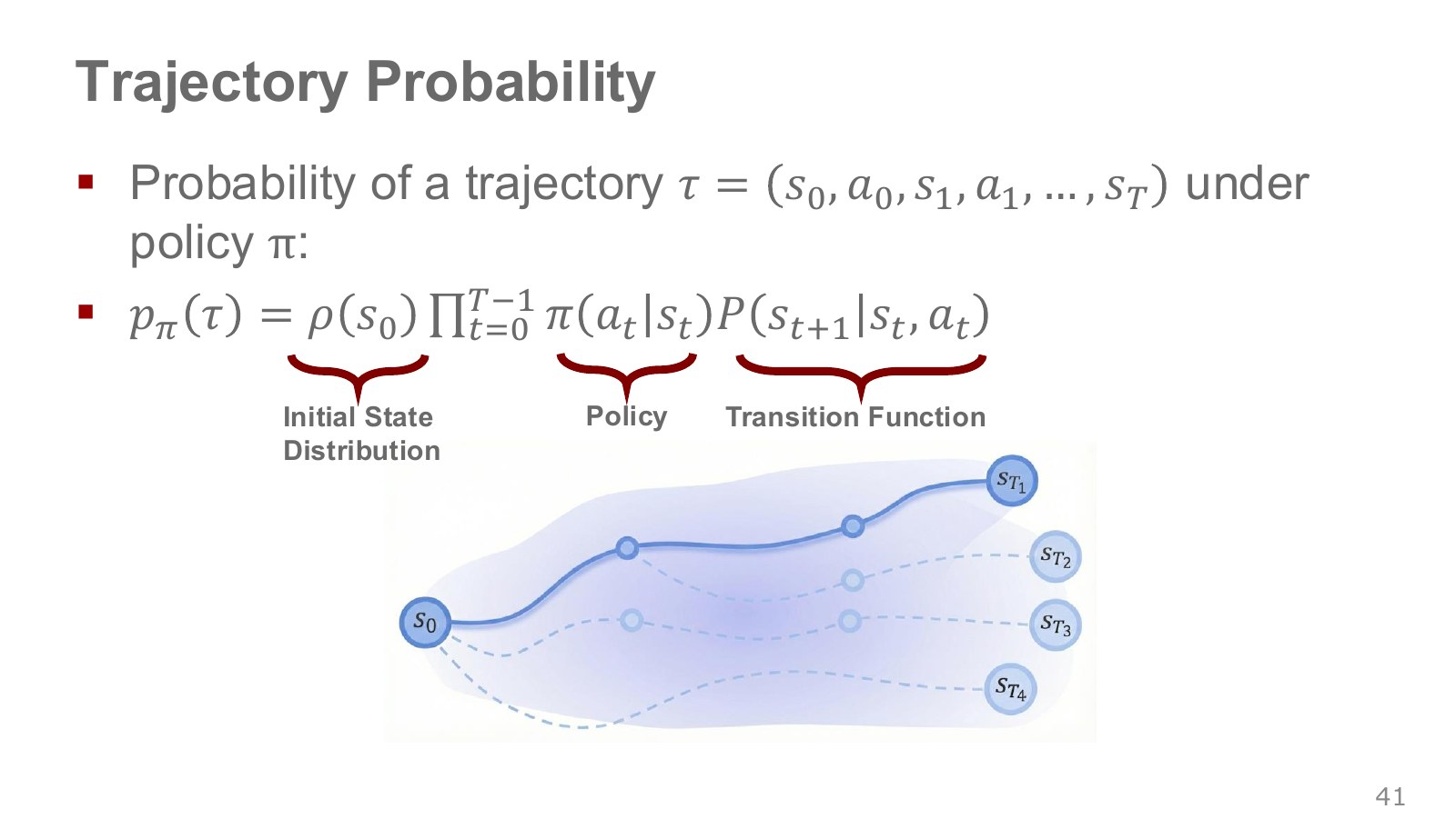
A trajectory records a sequence of actions and state transitions from an initial state. Write a record containing actions as . The slide’s product can be expressed with the same meaning as follows.
Explore the symbols and calculation A trajectory probability multiplies the initial-state probability by each step's action and transition probabilities
Read the equation in words
The probability of a trajectory is its starting-state probability multiplied successively by action-choice and environment-transition probabilities.
Understand each symbol
- One trajectory containing states and actions in time order. This symbol does not denote an angle.
- The distribution specifying an episode's initial state.
- A policy choosing actions given a state. A stochastic policy outputs probabilities or probability densities for actions.
- The probability of a next state after acting in the current state, or its density for continuous states.
- The number of steps or length of the action sequence considered here.
- Multiply every term in the indicated range. This appears when computing the joint probability of successive choices.
- Conditional notation: the information to the right of the bar is given. This is not a division sign.
Follow the calculation
- Begin with the initial-state probability.
- At each step, multiply by the policy's action probability and the next-state transition probability. For continuous variables, the expression denotes a density.
Check with a small example
A one-step trajectory with initial probability 0.5, action probability 0.4 and next-state probability 0.8 has probability .
An illustrative example for understanding the equation.
is the initial-state distribution, and means multiplying the stepwise terms. In a discrete illustrative example, an initial-state probability of 0.5, first-action probability 0.8, next-state probability 0.9, second-action probability 0.6 and final-state probability 0.7 give this particular trajectory probability 0.1512. This product uses successive probabilities conditioned on preceding states and actions, not an assumption that time steps are independent.
Changing only the policy changes the chosen actions and thus the trajectory distribution, even in an unchanged physical environment. Trajectory probabilities, 41:51–43:02. For continuous variables, interpret the expression as a probability density, distinct from the probability of one exact real-valued point. This expression describes a state-conditioned policy. A POMDP using observations must also account for observation generation and the policy’s dependence on history.
Specify what one transition covers. If a policy sets a target and receives its next observation after several lower-level control updates, its transition includes all intervening control and physics calculations. One simulator integration step and one policy decision need not represent the same unit.
Even on unchanged hardware, lower-level gains or action-hold duration can alter the transitions experienced by the policy. When comparing trajectory data, record command units, time intervals and execution controllers alongside state and action column names.
The branching paths below show that records can differ even from the same starting point. Initial states may be sampled differently, the policy may choose different actions, and the environment may produce different next states after the same action. The equation multiplies these sources of randomness in sequence. The inside the product represents one transition; the whole product describes the likelihood of a multistep record.
#P043 · Time limits and discount factors are part of the problem definition
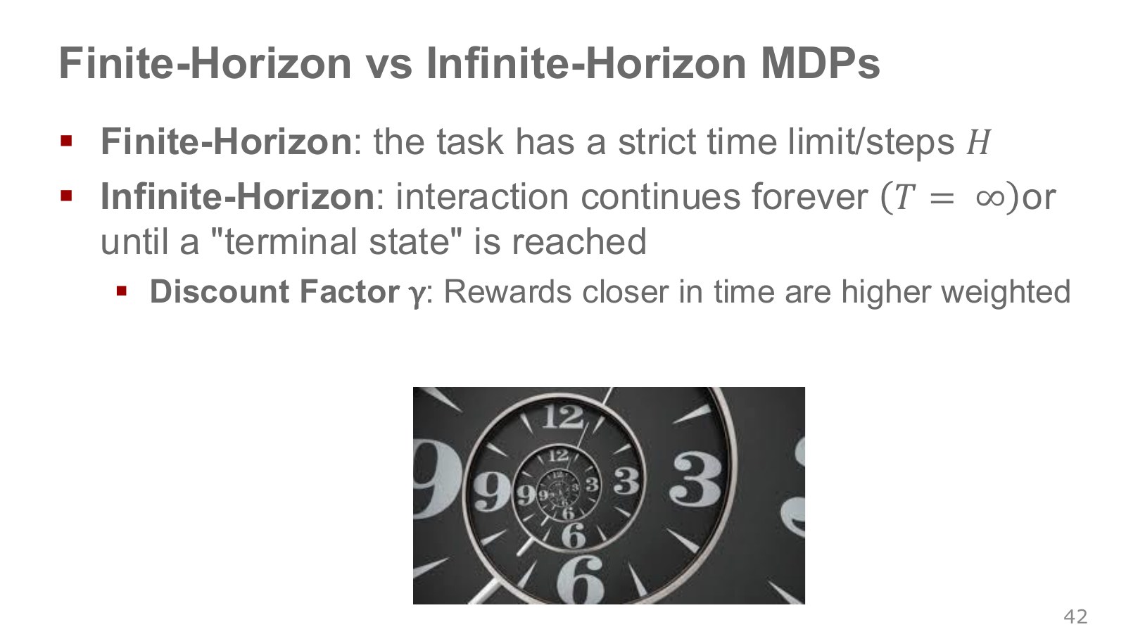
A finite-horizon problem requires completing the task within steps. At the same position, the best action can differ with 100 steps remaining versus one. Including remaining time in state or using a time-dependent policy expresses that difference.
For a problem with no preset stopping time, we can use a discount factor . With , more distant rewards receive progressively smaller weights. For bounded rewards, this can also make an infinite sum finite. considers immediate reward only; values nearer one give more weight to the distant future. An episode guaranteed to terminate may instead use an undiscounted sum with .
If a cup must be moved within five seconds, remaining time determines whether a long detour is feasible. A time limit can change optimal behavior, beyond being a runtime setting. Time-limit example, 43:06–44:47. Exercise APIs distinguish task termination (terminated) from an external time-limit cutoff (truncated). Running 200 steps should not itself be interpreted as success.
Control frequency and discounting also interact. At 10 Hz with , a reward one second ahead has weight . Switching to 100 Hz while retaining 0.99 gives a one-second weight of . Changing actions per second alone can substantially alter preferences over real time.
To match the discount weight after one second, convert the per-step discount factor as follows. This is an illustrative conversion for exponential discounting.
Explore the symbols and calculation Convert the per-step discount factor to preserve discount weight over the same physical time when the step interval changes
Read the equation in words
Adjust the step discount factor so that rewards decay by the same proportion over real time despite a changed control interval.
Understand each symbol
- The old and new per-step discount factors.
- The old and new physical step durations.
Follow the calculation
- Divide the new interval by the old interval.
- Raise the old discount factor to that ratio.
Check with a small example
If an old step lasts 0.1 seconds with factor 0.9 and the new step lasts 0.2 seconds, the new factor is . One new step covers two old steps.
An illustrative example for understanding the equation.
For the example above, . This alone does not make the full objectives identical across simulation settings. Reward accumulation and termination must also match, depending on whether a step reward represents a cost rate or a success event.
The Gymnasium explanation of time limits also distinguishes a finite horizon inherent to the task from an external rollout cutoff. When remaining time changes task outcomes, it belongs in the state representation. By contrast, an observation at an external evaluation cutoff should not automatically be treated as a terminal state of the original task.
#P044 · From a score on one run to the definition of a good policy
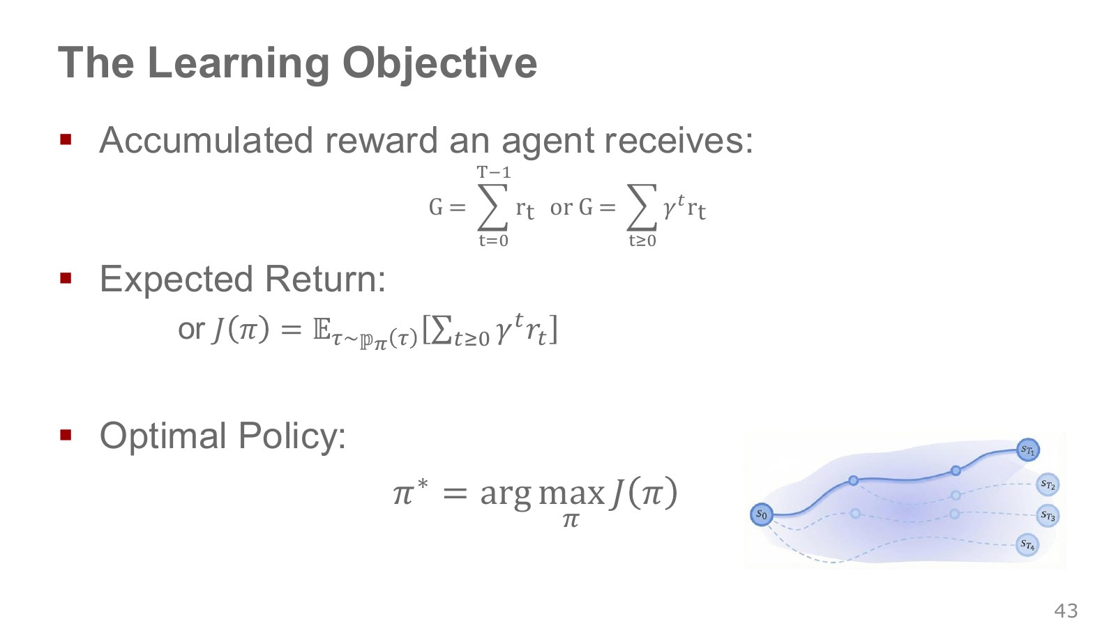
Under this chapter’s reward-index convention, the finite-horizon discounted return and policy objective are as follows. They connect the slide’s cumulative rewards, expectations and optimization in one notation.
Explore the symbols and calculation Define discounted reward sum as a trajectory's return and find a policy maximizing its expectation
Read the equation in words
Sum discounted rewards for one trajectory, then maximize the average across possible trajectories for the policy. A policy with the best expected return is optimal.
Understand each symbol
- One trajectory containing states and actions in time order. This symbol does not denote an angle.
- The reward received at one step: a learning signal defined so that larger is better.
- The discount factor for future rewards. Zero considers only the immediate reward, while values near one give more weight to the distant future.
- The number of steps or length of the action sequence considered here.
- A policy choosing actions given a state. A stochastic policy outputs probabilities or probability densities for actions.
- The performance measure given by a policy's expected return.
- A policy attaining the highest expected return.
- Add every term over the indicated range, computing one term and repeating through the end of the range.
- An expectation: an average over possible outcomes weighted by their probabilities.
Follow the calculation
- Multiply each trajectory reward by its time-dependent discount weight and sum.
- Average under the policy-induced trajectory distribution and compare policies to increase that average.
Check with a small example
Rewards 1 and 2 with discount factor 0.5 give trajectory return 2. If other trajectories are possible, their probabilities must also enter the average.
An illustrative example for understanding the equation.
is the score of one executed trajectory. is the expected return over possible trajectories generated by the starting state, policy and transitions. asks for a policy attaining the maximum, rather than the maximum score itself. The notation allows multiple optimal policies.
For three rewards and , the return is 0.81. An initial action scoring zero may have prepared the final success. In stochastic problems, one lucky successful run differs from a policy that performs well on average. The learning objective is a policy with high expected return, rather than one fortunate success. Objective function, 44:51–45:57.
Reward design carries through into this objective. Rewarding speed alone can omit collisions, and rewarding hand distance alone can omit actual grasping. A good policy is good for the problem objective we wrote down, so check whether that objective expresses the desired behavior before optimizing it.
While scores an entire policy, a value function asks for expected return from a particular state. In David Silver’s PDF, p. 28, starts from state and follows policy ; specifies first action and follows afterward. Distinguishing reward, one sampled return and expected return is the starting point for later algorithms.
This chapter defines the problem up to the meaning of an optimal policy. Writing a maximization expression does not by itself provide a way to compute that policy. The next chapter’s learning from demonstrations and the subsequent reinforcement-learning algorithms offer different ways to obtain policies with these inputs, outputs and objectives.
An expectation averages possible executions weighted by their likelihood. In a deterministic problem with the same success score every time, one run may equal that average. When starting states, actions or contact outcomes vary, multiple runs are needed. Here is a function scoring a policy, while the earlier IK was a matrix connecting joint and tool-tip changes. Reusing a letter can confuse their roles; check whether its input is a policy or joint configuration and whether its output is a scalar or a matrix.
#Inspecting observations, actions and rewards in a real simulation run
For a small example, I used Gymnasium’s Pendulum-v1, an environment that holds a single-joint inverted pendulum upright. The results below run a fixed PD controller initialized near the upright position. No parameters are trained from demonstrations or rewards.
The observation is , and the action is one torque between −2 and +2 N·. Representing the underlying state this way handles the angle’s periodic boundary. Reward is the negative of a cost combining weighted squared angle, angular velocity and torque. It is highest when upright, stationary and applying zero torque.
The experiment used seed=7, initial angles within ±0.2 rad and zero initial angular velocity to reproduce the same initial conditions. It compared zero torque with the following PD torque over 200 steps each.
Explore the symbols and calculation Compute PD torque from angle and angular velocity and clip it between minus 2 and plus 2 newton-meters
Read the equation in words
This fixed PD example applies torque opposing angle and angular velocity to restore the pendulum's reference pose. Clip the calculated torque when it exceeds actuator limits.
Understand each symbol
- Pendulum angle and angular velocity. Theta here is not a neural-network weight.
- The control torque applied to the pendulum.
- An operation limiting values below the lower bound or above the upper bound to those bounds.
Follow the calculation
- Multiply angle by −15 and angular velocity by −3, then add.
- Clip the result to −2 through 2 Nm. These are example gains, not universal robot settings.
Check with a small example
Angle 0.1 rad and angular velocity 0.2 rad/s give −2.1 Nm, so the applied command is clipped to −2 Nm.
An illustrative example for understanding the equation.
The clip function restricts a result to specified lower and upper bounds. This controller demonstrates stabilization near upright. The result does not establish swing-up from the downward position.
| Fixed control method | Reward sum over 200 steps | Final angle (rad) |
|---|---|---|
| Zero torque | -502.751685 | 0.159858 |
| PD | -0.019170 | 0.000000 |
At step 200, both runs reported terminated=False and truncated=True. They reached the default time limit rather than ending on a task-success judgment. The reward sum is an undiscounted rollout return for this one initial condition, not expected performance across starting states or a comparison of RL algorithms.
The core execution sequence is to form a command from the observation, pass it to step, and receive a new observation and reward. Fixing the seed in reset specifies reproducible initial conditions.
import gymnasium as gym
import numpy as np

env = gym.make("Pendulum-v1")
obs, info = env.reset(seed=7, options={"x_init": 0.2, "y_init": 0.0})
for _ in range(200):
    theta = np.arctan2(obs[1], obs[0])
    torque = np.clip(-15.0 * theta - 3.0 * obs[2], -2.0, 2.0)
    action = np.array([torque], dtype=np.float32)
    obs, reward, terminated, truncated, info = env.step(action)
    if terminated or truncated:
        break
env.close()
The executable files, environment versions, CSVs and numerical checks are public together. They include checks of coordinate transformations, the two IK solutions for a 2R arm, numerical differentiation of the Jacobian gradient, quintic boundary conditions, PID calculations, trajectory probabilities and returns. The additional file supplement_checks.py contains eight numerical checks covering pseudoinverse/DLS behavior at singular configurations, inverse transformations, policy-induced transition mixtures, action ranges and discount-factor conversion.
#Continue with robot-arm exercises
The official ETH HW2 connects this chapter in three stages: convert spatial targets into joint configurations through IK, add trajectory generation and control, then train a policy in a MuJoCo environment.
| Official exercise | Connection to examine | What to read before running |
|---|---|---|
| Exercise 1 | Target point → IK → joint configuration | Directly changing poses for visualization differs from physical tracking control. |
| Exercise 2 | Quintic trajectory → IK → PID → physics simulation | Inspect target-versus-measured joint errors, gains and the meaning of output commands. |
| Exercise 3 | Observation → policy action → actuator → next observation and reward | Inspect the mapping from normalized actions to physical targets. |
The official description sets Exercise 3’s policy at 10 Hz and physics at 500 Hz, with 50 physics steps per policy action. Exercise 2 interprets data.ctrl as torque input, while Exercise 3 interprets it as joint targets. A variable name can have a different meaning under a different loaded actuator model. The table is a guide to reading the public assignment and code; it does not report training the official SO-101 assignment or operating a real robot here.
For larger parallel simulation environments, continue with the official NVIDIA Isaac Lab tutorial. Learning to identify the boundaries among observations, actions, physics and rewards before scaling up makes the structure easier to follow as settings change.
Chapter 03 turns to imitation learning: learning a policy from expert behavior before starting reward-based trial and error. The difficulty of taking observation-to-demonstrated-action learning into actual execution connects directly to this chapter’s sequential decision-making.
#Sources and further reading
- Oier Mees — ETH Robot Learning, Lecture 2: Robot Control & MDPs · Lecture video, 2026-02-23 · Slides
- Lecture-slide image copies. P numbers follow the file order in this copy. Administrative, transition-only and closing slides are omitted.
- Lynch and Park — Modern Robotics: rigid bodies and links · Six joint types and degrees of freedom · Configuration-space shapes · Task space and workspace
- Lynch and Park — Modern Robotics: homogeneous transformations · Time scaling. Videos are accompanied by official scripts.
- Hado van Hasselt — DeepMind × UCL 2021, Introduction to RL · Lecture PDF
- Modern Robotics — Numerical inverse kinematics · PD/PID torque control under gravity
- David Silver — UCL 2015, original MDP lecture PDF · Public Google DeepMind lecture video · Author’s lecture materials and terms of use
- NVIDIA Isaac Lab — Differential IK · MuJoCo — Actuator settings
- Hung-yi Lee — NTU RL introduction · Reward design and imitation learning
- Farama Foundation — Gymnasium Pendulum documentation · Original ETH HW2 code
Copyright in the lecture slides belongs to Oier Mees and the respective rights holders. Figures and photographs from Modern Robotics, ABB, Latombe, LaValle and others belong to their original creators. The explanatory 2R arm, reward and probability calculations, and directly generated graphs in these notes are separate examples developed to explain the concepts.