If we collect a driver’s road images and steering commands, can a robot learn to drive from them? The starting point is supervised learning with inputs and targets. But a robot’s answer changes the next scene it sees. Let us examine learning actions from demonstrations, then three difficulties that emerge during actual execution.
Oier Mees · ETH Zurich 2026, Lecture 3 · Official course · Original PDF
#P001 · Learning a rule for action from demonstrated movement
Chapter 02 converted desired tool-tip positions into joint targets and control commands, then described decision-making through states, actions, transitions and rewards. Now we ask how to obtain the policy within that framework.
Imitation learning is a family of methods using expert behavior as a learning signal. Human teleoperation records or runs from an existing controller can serve as demonstrations. Instead of beginning with reward-based trial and error alone, the main methods here start by predicting what the expert did in the same situation. Demonstrators need not always be optimal, so data quality and coverage matter too.
#P003 · Reconnecting observations, policies and actions over time
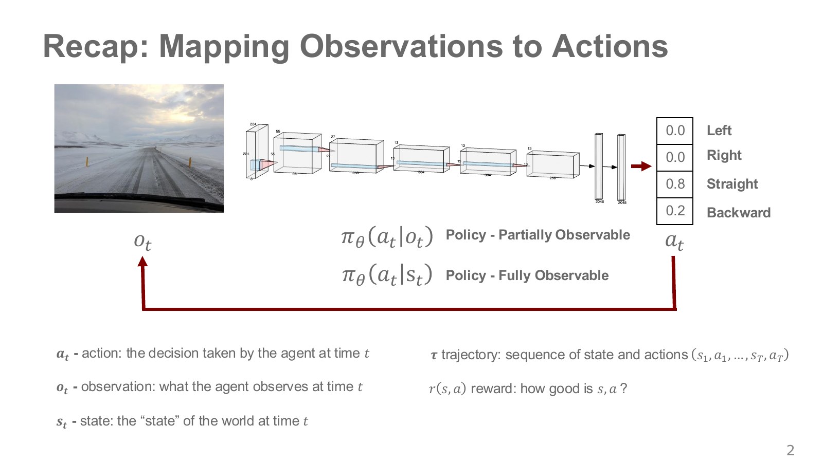
The road image is an observation; a steering command is an action. Information needed to predict what happens next, including the car’s actual position, velocity and heading, is modeled as state. One camera image need not reveal all of it.
Network weights define the action-selection rule. is the probability or density assigned to action given observation at step . The bar denotes conditioning on given information. With access to full state, we can condition on instead of the observation.
The red arrow below the figure traces actions through a changing environment and back to the next image. The 0.8 above it is a probability of choosing forward, not a success rate. A wrong steering action changes the next camera view. Predicting actions in stored images and completing a task through repeated action therefore need separate evaluation. Original lecture, 2:09–2:49.
#P004 · What should a demonstration record contain?
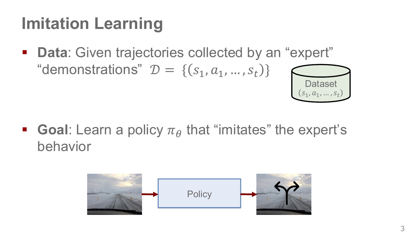
A demonstration records what an expert observed and did while performing a task. A trajectory is one run linking states and actions, or observations and actions, in time order. A collection of runs forms dataset .
For cup grasping, the record can synchronize camera images, joint measurements, gripper commands and arm commands. Video alone, without corresponding executable robot actions, does not immediately provide the input–target pairs needed for basic behavior cloning. Mapping a video of a human grasp to robot-joint torques remains a separate problem.
For training, split trajectories into observation–expert-action pairs . The asterisk marks an expert-provided target here, not a mathematically proven optimum. Pairing an image with an action taken 0.1 seconds too late, for example, misaligns the response timing to be learned. Original lecture, 2:41–3:54.
NTU’s imitation learning lecture, 5:26–7:51 likewise connects driving records and arm demonstrations through observation–action learning. This offers a starting point when rewards are difficult to design. But the goal “move it” does not establish command units: first specify whether the records contain position targets, displacements, velocities or torques.
#P005 · Behavior cloning: reducing the error between predictions and expert actions
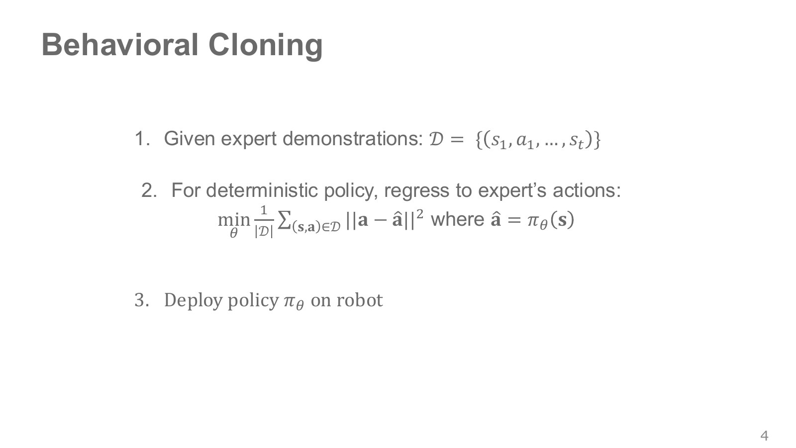
Behavior cloning (BC) turns demonstrations into supervised training data for a policy. Supervised learning finds a prediction rule from input–target pairs. A deterministic policy predicting one continuous action can be framed as regression: predicting numerical values.
Explore the symbols and calculation Behavior-cloning MSE: average the squared difference between predicted and expert actions over the dataset
Read the equation in words
Square and average component-wise differences between model and demonstrated actions. This basic behavior-cloning loss moves predictions toward targets.
Understand each symbol
- The policy's predicted action. A hat marks an estimate, distinct from the demonstrated target.
- The target action demonstrated by the expert for that observation. The asterisk is not multiplication.
- The sensor observation at step . It is not assumed to equal the full physical state.
- The parameters collecting the trainable weights of the network or policy.
- The number of data points or samples being averaged. Dividing the sum by this count gives a per-sample average.
- A loss quantifying the difference between a prediction and a target. Learning or optimization aims to reduce it.
- Add every term over the indicated range, computing one term and repeating through the end of the range.
- The squared length obtained by squaring and summing all vector components. It combines coordinate-wise errors into one nonnegative quantity.
Follow the calculation
- Compute the predicted action for every observation.
- Square and sum component-wise differences from targets, then divide by the sample count.
Check with a small example
Errors 1 and −2 for two demonstrations give loss . Squaring prevents positive and negative errors from canceling.
An illustrative example for understanding the equation.
counts observation–action pairs. The hat in marks the predicted action; is the demonstrated action. Squaring a vector norm means squaring and adding component-wise action differences. We adjust weights to reduce the resulting average, the mean squared error (MSE).
Training repeatedly samples small groups of pairs called minibatches, predicts actions with the network, differentiates the loss with respect to its weights, and updates them. Computing these derivatives backward through the network is backpropagation. Original lecture, 3:56–5:01.
When predicting an action distribution rather than one value, we can reduce the following negative log-likelihood (NLL) to give demonstrated actions high probability or density.
Explore the symbols and calculation A stochastic policy reduces negative log-likelihood to increase the likelihood assigned to demonstrated actions
Read the equation in words
Train the policy to assign high probability or density to actions actually demonstrated. Lower likelihood for the target action gives larger negative-log loss.
Understand each symbol
- A policy that maps an observation to an action distribution. The subscript denotes the weights that define it.
- The target action demonstrated by the expert for that observation. The asterisk is not multiplication.
- The number of data points or samples being averaged. Dividing the sum by this count gives a per-sample average.
- The parameters collecting the trainable weights of the network or policy.
- Add every term over the indicated range, computing one term and repeating through the end of the range.
- The natural logarithm. It converts products into sums and is defined only for positive inputs.
- Conditional notation: the information to the right of the bar is given. This is not a division sign.
Follow the calculation
- Obtain the policy probability of the target action.
- Negate its natural logarithm and average over the dataset.
Check with a small example
A discrete target-action probability of 0.5 gives loss about 0.693; 0.9 gives about 0.105. Continuous densities can exceed 1, so negative log-density can be negative.
An illustrative example for understanding the equation.
Likelihood assesses how much probability or density a model assigns to the observed actions. Logarithms make products across steps easier to handle as sums, and the minus sign converts maximization to minimization. For continuous actions, distinguish density from the probability of one exact real-valued point. Combining components with different units, such as torque and distance, also changes their loss contributions, so inspect normalization and weights.
#P006 · Why a small action error changes the next input
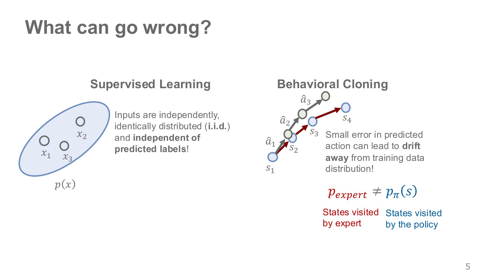
The points in the left oval are fixed inputs. Classifying a photograph as a cat or dog does not change the next photograph’s pixels. On the right, the gray expert path and the executed policy path diverge after a small action error. Moving somewhere slightly different changes the next input from the one the expert saw.
Distribution shift is a difference between training-input and execution-input distributions. Alongside external changes such as weather, here the policy’s own actions change its input distribution. A car drifting out of its lane, seeing a less familiar image and steering incorrectly again illustrates compounding error.
Write the expert’s and learner’s state-visitation distributions as and . They can differ even when both start on the same road. These distributions describe how often states are visited, distinct from probabilities of selecting actions. Original lecture, 5:38–8:44.
i.i.d. means samples are independent and identically distributed; it does not mean inputs and targets are unrelated. Supervised learning aims precisely to learn their relationship. The key difference is a closed loop in which predictions change future inputs. Consecutive demonstration frames are correlated too, so shuffling frames alone does not solve the distribution mismatch between training and execution.
#P007 · NVIDIA's camera-based steering: behavior cloning in practice
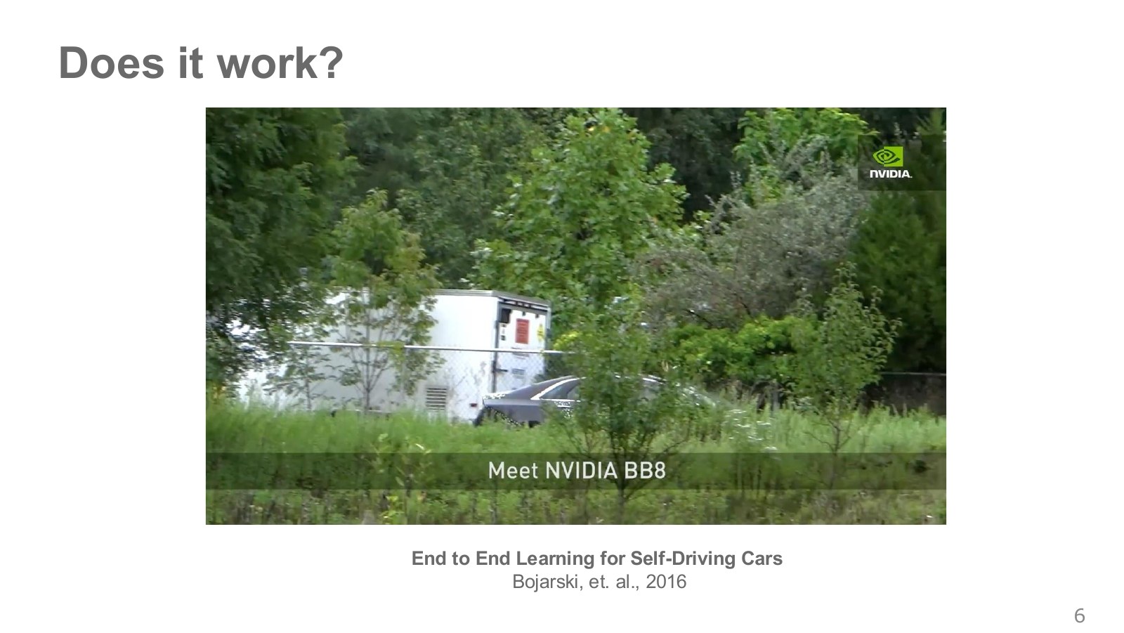
NVIDIA’s 2016 DAVE-2 study trained a neural network to predict steering commands from forward-facing camera images. Instead of hand-writing every intermediate rule about road boundaries and vehicle state, it learned from image–steering pairs recorded during human driving. The photographed vehicle demonstrates this approach on a real car. Original lecture, 8:50–9:53.
End-to-end here describes learning the connection from image input to steering output. It should not be expanded into a claim that one network handled acceleration, braking, destination selection and every safety decision. The paper studies a steering system under specified training and evaluation conditions. Original NVIDIA paper.
How, then, did it address compounding errors in unfamiliar states? An important connection is teaching recovery from off-center positions, rather than including only examples of good centered driving.
#P008 · What centered lane-following records do not teach
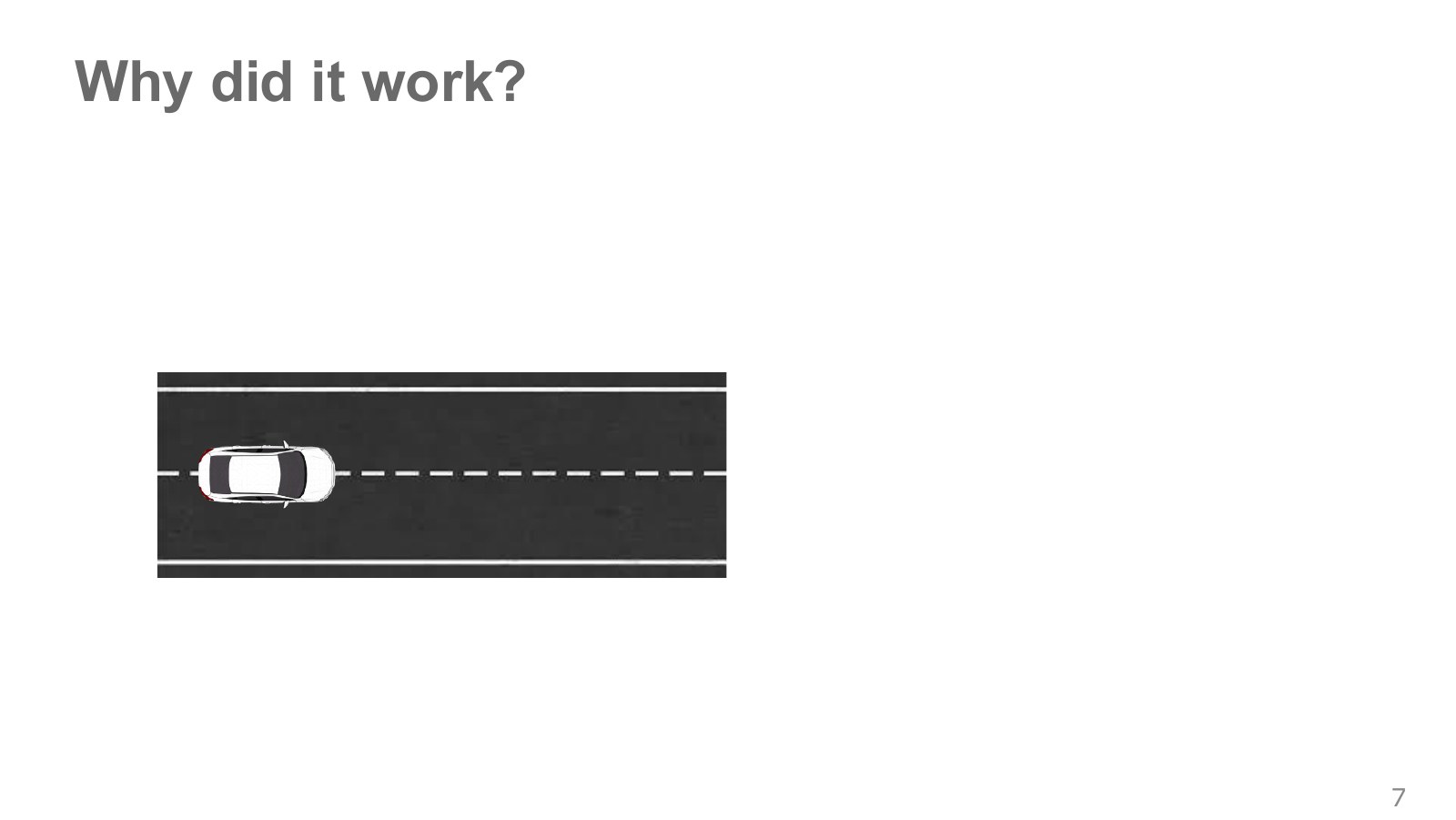
Imagine a car viewed from above, traveling straight along the lane center. Its expert command may be almost straight ahead. Thousands of similar images and actions can thoroughly cover that centered-driving relationship.
Record count and situation coverage are different. Adding only accurately centered driving can still leave no examples of recovering rightward from the left lane edge. The policy needs more than replaying demonstrated paths: it must choose the right next action from a slightly off-course current state. Original lecture, 10:03–10:53.
#P009 · An angled, off-course car needs target recovery actions
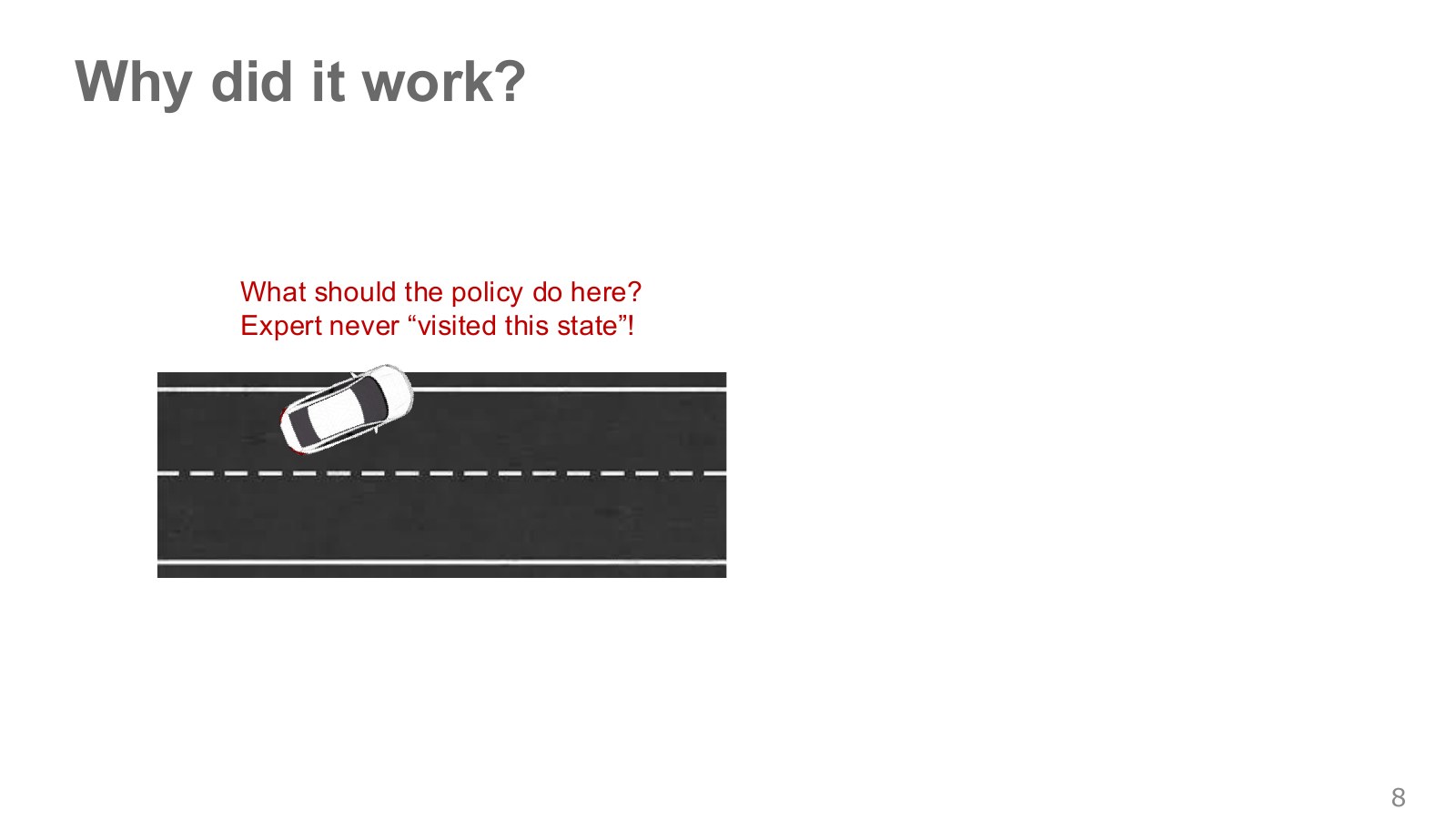
Now the vehicle has drifted and turned obliquely to the lane. The image differs from centered driving, and the required steering differs from straight ahead. Fitting familiar centered images does not establish that the policy has learned recovery.
Adding this state to training requires both its image and a target action specifying which way and how far to steer to recover. More examples of bad situations alone differ from records pairing those situations with good corrective behavior. Original lecture, 10:55–11:59 · NTU on situations outside demonstrations, 8:00–9:01.
#P010 · Data augmentation changes the image and recovery action together
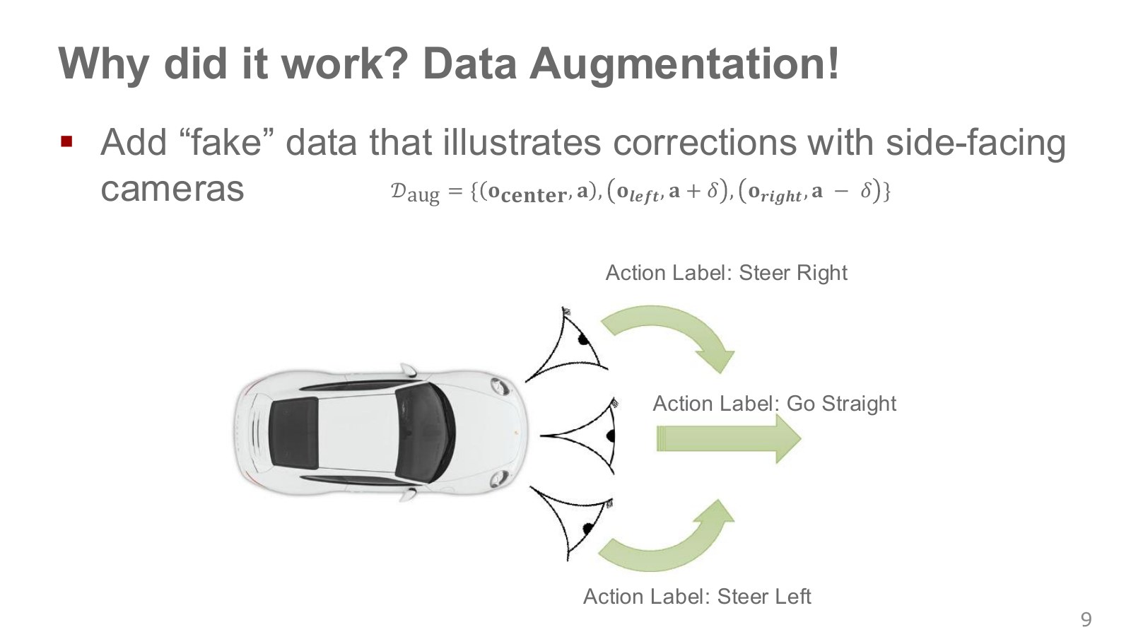
Data augmentation applies valid transformations to existing data to broaden training cases. For driving, side-camera images can supplement the central view with scenes that appear off-center. Their target actions must also be adjusted to steer back toward the center.
The illustrative expression below takes right steering as positive and writes correction magnitude as . A left-offset view is paired with rightward recovery, and a right-offset view with leftward recovery.
Explore the symbols and calculation Illustrative augmentation: changing camera viewpoint also adjusts steering targets toward recovery in the opposite direction
Read the equation in words
When generating changed camera views, also adjust the steering target needed in each scene. Changing inputs alone can create incorrect input–target pairs.
Understand each symbol
- The central, left and right camera observations.
- The original steering and the steering correction for the viewpoint change.
- The set of augmented observation–target-action pairs.
Follow the calculation
- Prepare images from central, left and right viewpoints.
- Add or subtract the steering correction needed to return toward the central path and pair it with each view.
Check with a small example
Original steering 0 and correction magnitude 0.1 can give targets 0, +0.1 and −0.1. Actual signs depend on camera placement and steering coordinates.
An illustrative example for understanding the equation.
denote central, left and right camera observations. Signs depend on the steering convention. This does not assert that one constant correction works accurately for every vehicle; camera position, orientation and the desired recovery path matter.
The original NVIDIA training diagram draws image translation/rotation and steering-target adjustment as separate boxes. Moving only the image while retaining its old steering target can teach an incorrect correspondence.
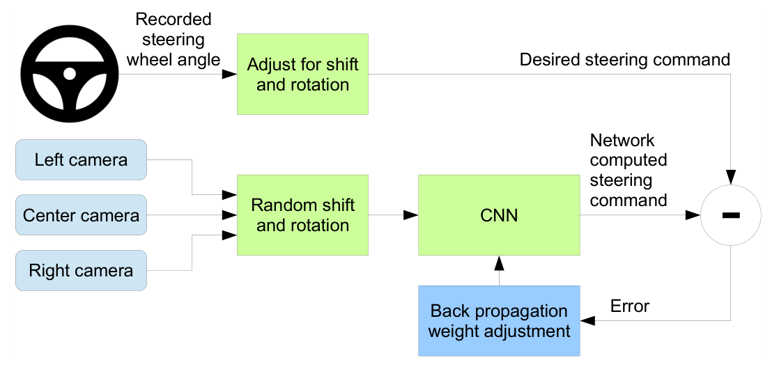
A CNN is a convolutional neural network that computes spatial image features. The backpropagation arrow traces the training path that updates weights from prediction–target differences. Distinguish training with multiple cameras and transformed images from execution using the central forward camera. Original lecture, 12:01–13:03.
#P011 · Learning a flight direction from a person walking a forest trail
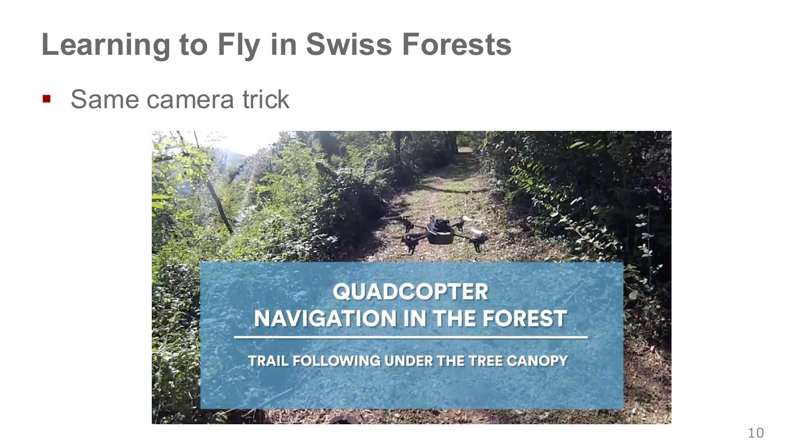
In the forest-trail example, a person walks with head-mounted cameras facing centrally, left and right. The central camera records views aligned with the trail, while the side cameras supply apparently misaligned views. Pairing them with straight, left-turn and right-turn labels trains a direction classifier for following the path.
Labels derived from those three views specify direction. A real drone still needs separate flight control to convert a chosen direction into attitude and thrust.
The person did not directly demonstrate every drone-motor command while walking through the forest. Camera directions and the assumption that the person follows the trail provide a way to construct target direction choices. The image-to-direction network is distinct from the lower-level controller stabilizing the aircraft.
Giusti et al.’s original paper explains three-camera collection, augmentation that reverses labels when images are flipped horizontally, trail classification and ground/flight evaluation. Its results do not establish navigation through every pathless forest or avoidance of every obstacle. Original paper · Original lecture, 13:12–15:06 · Berkeley on the same collection principle, 2:44–5:06.
#P012 · A bound examines worst-case accumulation, not the error a robot will necessarily make
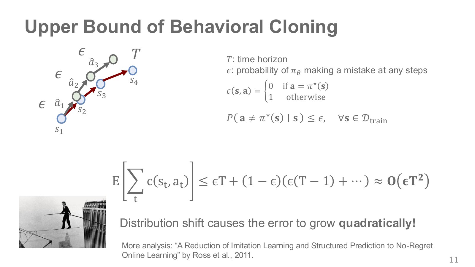
Even a small probability of one incorrect action can lead to a large task-level loss if the robot then remains in unfamiliar states. The tightrope illustration represents a failure affecting every remaining step.
Let be the number of execution steps and a small action-error rate on expert-visited situations. Consider a simple model with per-step cost 0 or 1 and cost 1 at every remaining step after leaving the expert path. Departure at the first step incurs cost for steps; first departure at the second incurs it for steps.
Explore the symbols and calculation An early error can incur cost over every remaining step, giving intuition for quadratic worst-case accumulation in the horizon
Read the equation in words
If an early error damages many later steps, worst-case accumulated error cost can grow quadratically with the horizon.
Understand each symbol
- The length of a trajectory or sequence. Here it sets how many steps enter the sum or product.
- A small per-step error rate under the expert's state-visitation distribution.
- The asymptotic growth order of a bound, not an exact equality or probability itself.
- Add every term over the indicated range, computing one term and repeating through the end of the range.
Follow the calculation
- Count the first error's impact through all remaining steps, down to one step for the last error.
- Multiply the sum from 1 through the full horizon by the per-step error rate.
Check with a small example
Horizon 4 and error rate 0.1 give . This does not equal the failure probability of every actual policy.
An illustrative example for understanding the equation.
The sum conservatively combines these effects as an intuition. describes asymptotic growth in ; it does not predict that BC always worsens quadratically in experiments. If each step costs at most 1, actual total cost cannot exceed , so a large upper bound may become uninformative.
In a separate calculation with pre-departure error probability fixed at 0.01 per step and no recovery after departure, gives expected cost about 1.9728. The simple sum above gives 2.1, covering it. Independent, isolated errors costing only one step each would instead give 0.2. Comparing these models reveals what it means for an error to affect the remaining horizon.
Page 2 of Ross et al.’s original paper develops general bounds under assumptions including imitation error on the expert distribution and bounded task costs. Do not apply a 0–1 error count blindly to the probability that continuous torque matches an expert exactly. Assumptions are needed to connect action error to task cost. Original lecture, 15:11–18:00 · Berkeley’s tightrope calculation, 6:45–10:40.
#P013 · Labeling the states the learner actually visits with good actions
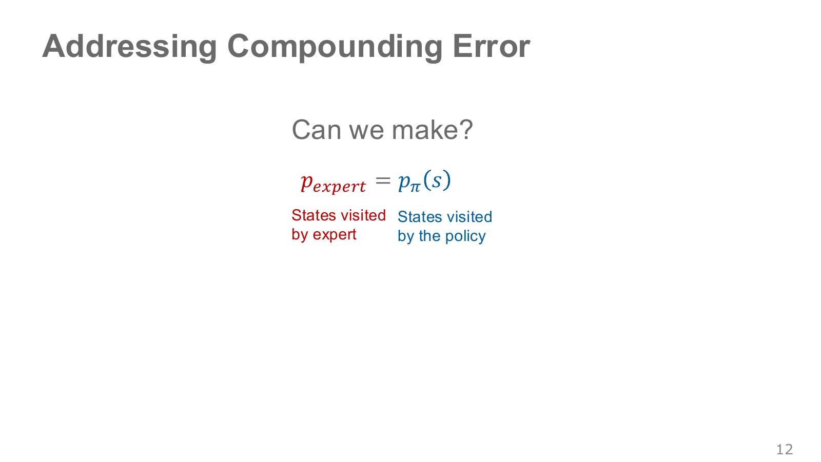
If a policy repeatedly fails in states missing from its data, those states can be brought into training. Shift the question from whether it followed the expert’s path to what the expert would do here, where the current policy has arrived.
The equality sign between distributions in the figure expresses the aim of reducing this gap. It does not say that every state’s visitation frequency must match perfectly before learning is possible. It addresses the lack of useful targets in states the learner frequently encounters. This makes the next algorithm’s collection sequence clearer. Original lecture, 18:03–18:40.
#P014 · DAgger: alternate policy rollouts and expert labeling
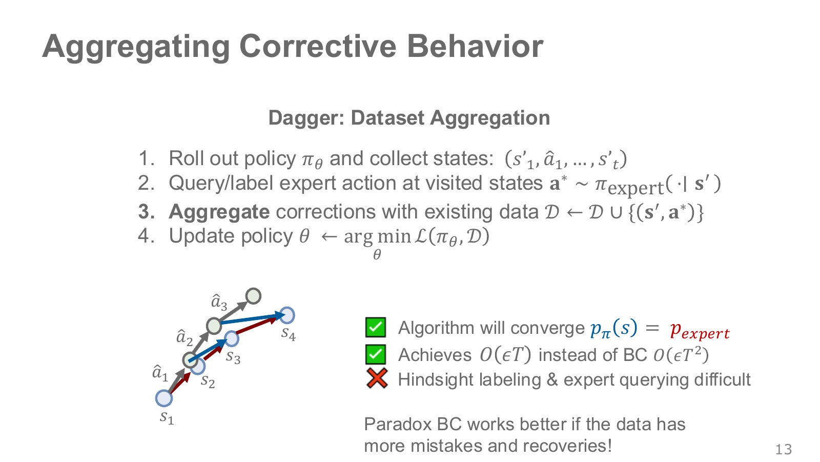
DAgger stands for Dataset Aggregation. It begins with a policy trained on expert demonstrations, then collects states visited by the learned policy and asks the expert for the appropriate actions there.
- Execute the current policy and record the states visited. Running a policy in an environment to collect such a record is a rollout.
- Obtain the action the expert would choose at each visited state.
- Add the new state–expert-action pairs to the existing dataset.
- Retrain on the aggregated data and repeat.
Explore the symbols and calculation DAgger labels states visited by the current policy with expert actions and aggregates them with the existing dataset
Read the equation in words
Ask an expert for correct actions at states actually visited by the current policy and add them to existing data, including recovery from the demonstration path.
Understand each symbol
- The training dataset. What one item contains is specified by the equation.
- The state at step , containing information such as position and velocity needed to predict what happens next.
- The target action demonstrated by the expert for that observation. The asterisk is not multiplication.
- The current policy executed at round .
- The updated dataset and the union combining existing and new records.
Follow the calculation
- Run the current policy and collect visited states.
- Obtain expert actions there, aggregate the pairs with existing data and retrain.
Check with a small example
If the expert data contains only 100 centered-driving examples, add learner-visited states off to the left with corrective steering labels.
An illustrative example for understanding the equation.
indexes data-collection and training rounds. The procedure does not copy the learner’s mistaken action as a target; it labels the state reached through that action with a good expert action. Retaining older data covers both previously familiar states and new recovery states. The blue correction arrow illustrates this additional learning.
The original algorithm also includes mixtures of expert and learner policies during collection and conditions on learning and policy selection. Its theoretical point is to address imitation loss under policy-induced state distributions. The equality drawn in the figure is not an unconditional guarantee that every neural network exactly reproduces the expert’s visitation distribution. Linear-order performance guarantees likewise depend on the imitation loss and assumptions about cost and recovery. Original paper, pp. 3–4.
When we say that data containing mistakes can help, the valuable part is the correct recovery after the mistake. Simply adding more incorrect actions can change what the model learns. Labeling joint torques individually from static robot images is also difficult for a person. That cost motivates the next intervention approach. Original lecture, 18:44–20:27.
#P015 · Human-Gated DAgger: a person takes over when needed
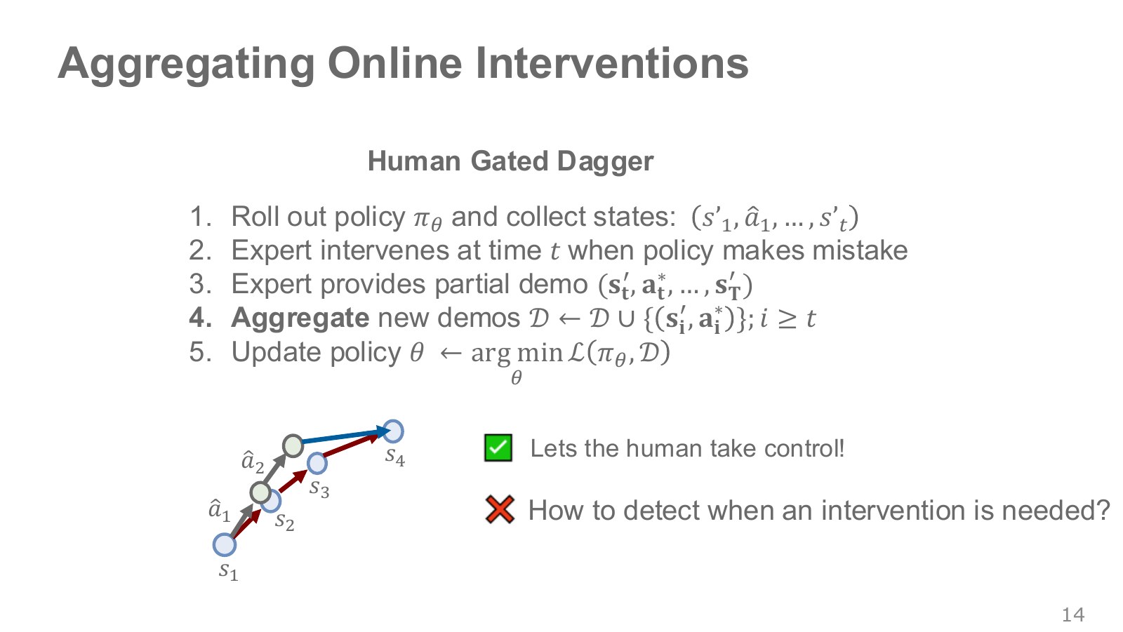
An intervention is a person taking over policy execution to demonstrate a segment. Think of a driving instructor taking the wheel at a necessary moment, instead of driving the whole route for the learner.
In Human-Gated DAgger, a person watches execution, takes control when trouble appears, and adds observation–action records from the recovery segment as new demonstrations. This can reduce the burden of separately labeling every past frame, but it collects a different distribution from basic DAgger, which queries targets at all visited states.
Questions remain about when to intervene, how to join commands before and after takeover, and how to discover errors in unsupervised stretches. A high policy probability does not guarantee a situation warrants confidence. Separate recognizing a difficult moment from learning what to do then. Original lecture, 20:32–22:25.
#P016 · Recognizing ambiguity and asking the person again
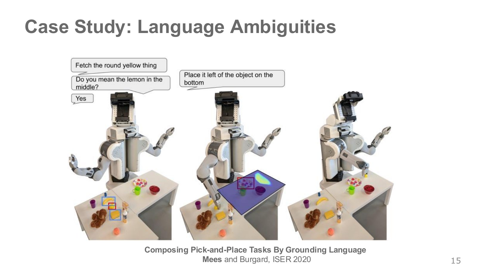
“Bring the round yellow object.” With several yellow objects on the table, uncertainty about which object is meant comes before choosing a gripper movement. The boxes in the photograph mark candidate object regions for the instruction.
The robot can ask a distinguishing question, such as “Do you mean the lemon at the bottom center?”, and act after the answer. Relative descriptions such as “left of the lower object” also need their reference object established. Connecting language to a visual referent is language grounding.
Here the robot asks for missing task information instead of asking an expert to specify every motor command again. It connects to detecting a need for intervention, but is not itself a universal detector of robot failures. Original lecture, 22:30–23:15.
#P017 · Learning candidate scores and a basis for asking questions
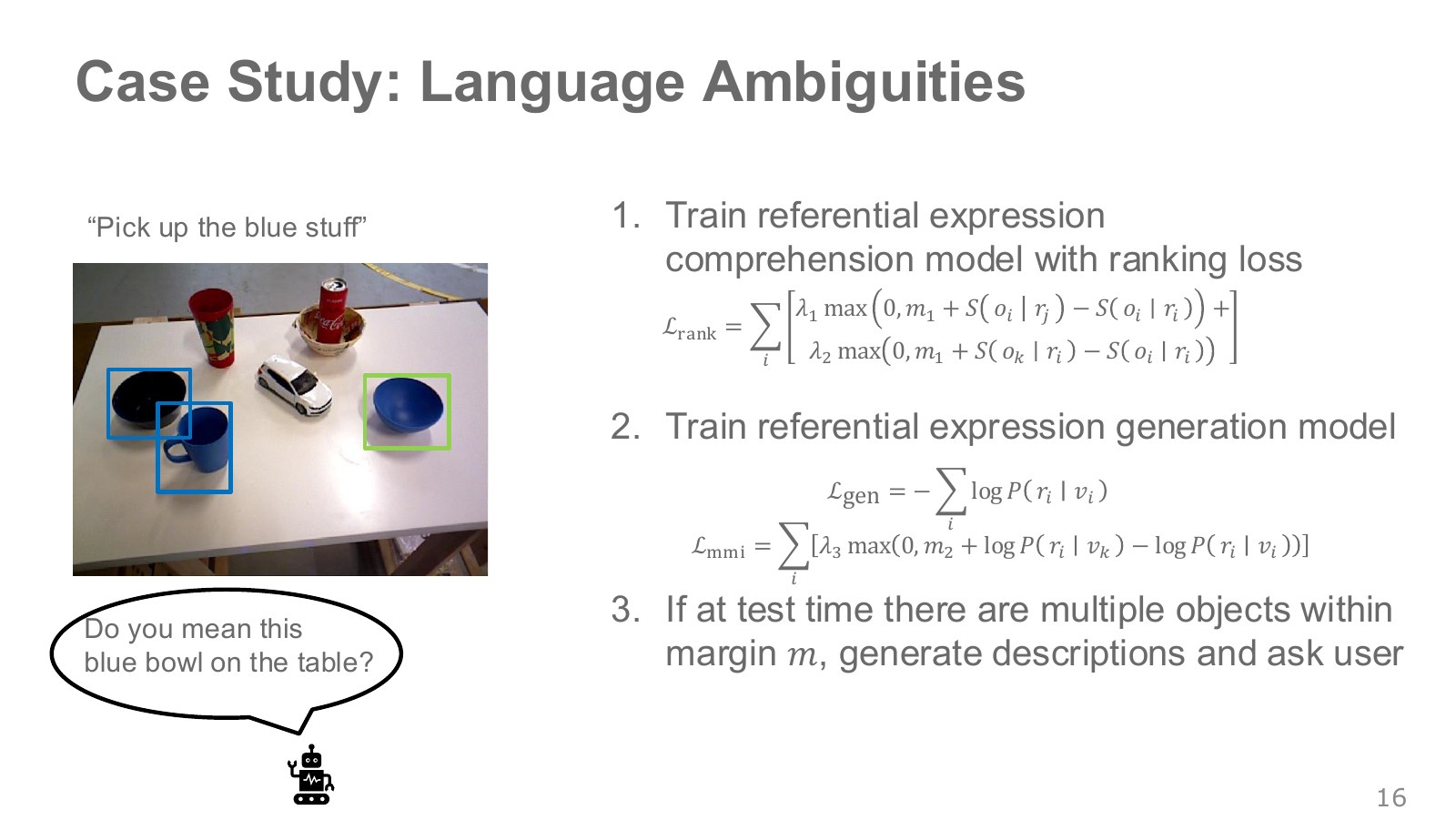
For “pick up the blue one,” a blue bowl and a blue cup may both be candidates. A referring-expression comprehension model scores how well a sentence matches each object. Here is the correct object, the referring sentence and their compatibility score. The symbol in this section denotes a sentence, not reward.
Require the correct pair’s score to exceed an incorrect pair’s score by at least . This minimum difference is the margin. Split the original ranking loss into two terms for one correct pair as follows.
Explore the symbols and calculation Ranking loss makes the correct object–sentence pair outscore incorrect sentence or object pairings by a margin
Read the equation in words
Raise the correct pair's score above incorrect pairs by a specified gap. A comparison incurs no penalty when the gap is already sufficient.
Understand each symbol
- The score for a correct sentence–object pair. Here is a referring sentence, not reward.
- Incorrect candidate objects and sentences, respectively.
- The required score margin and weights on the two comparison terms.
- Conditional notation: the information to the right of the bar is given. This is not a division sign.
Follow the calculation
- Add the margin to an incorrect score and subtract the correct score.
- Retain positive shortfalls only, then weight and add the two kinds of incorrect-pair comparison.
Check with a small example
Correct score 3, incorrect score 1 and margin 1 give . An incorrect score of 2.5 gives penalty 0.5.
An illustrative example for understanding the equation.
The first line pairs the same object with an incorrect sentence ; the second pairs the same sentence with another object . weights the two penalties. sets the penalty to zero when the gap is sufficient and penalizes only the shortfall. A correct score of 0.8, incorrect score 0.4 and margin 0.2 give zero penalty; an incorrect score of 0.7 leaves a 0.1 margin shortfall. These numbers are a separate illustration of the structure.
Asking a question also requires generating a description that distinguishes candidates. If contains visual features of an object and its surroundings, a generation loss can favor the actual description while a discriminative term discourages confusion with other objects.
Explore the symbols and calculation Sentence generation favors the correct object's description and penalizes descriptions fitting other objects similarly well
Read the equation in words
Learn both to generate an appropriate sentence and to prevent it from indiscriminately matching other objects.
Understand each symbol
- The correct sentence, target-object representation and alternative-object representation.
- The generation loss and the comparison loss separating correct from incorrect pairs.
- The comparison margin and its penalty weight.
- Add every term over the indicated range, computing one term and repeating through the end of the range.
- The natural logarithm. It converts products into sums and is defined only for positive inputs.
- Conditional notation: the information to the right of the bar is given. This is not a division sign.
Follow the calculation
- Calculate the target sentence's negative log-likelihood for the correct object.
- Add a margin penalty when the sentence also has high likelihood for another object.
Check with a small example
Correct/incorrect object log-likelihoods −1 and −3 with margin 1 give no comparison penalty. Incorrect log-likelihood −1.2 leaves an unweighted penalty of 0.8.
An illustrative example for understanding the equation.
weights the discriminative term, and is the required log-likelihood gap between the correct object and others. The first term encourages good descriptions; the second reduces their equal fit to other candidates. For example, “the blue bowl on the right side of the table” can distinguish candidates better than “the blue one.”
At execution time, close candidate scores can inform a decision to ask. A small score gap is not an exact failure probability: scores are comparative model signals and should not be treated as probabilities without validation. The original ranking expression raises correct-pair scores, so I read the difference between its two scores rather than relying on the sign described verbally. Original lecture, 23:15–24:40.
#P018 · Question, confirmation and execution form one interaction
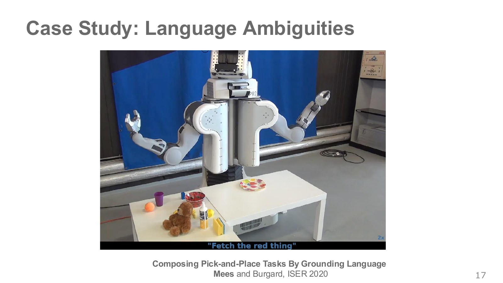
In the robot interface, a spoken instruction is followed by candidate selection, confirmation when needed—“Do you mean the banana in the middle?”—and grasping and transport. A person’s answer supplies new information narrowing an ambiguous goal. Only after that goal is specified can the system decide the arm actions needed to execute it.
Candidate names and positions help distinguish them when forming a question. With two bananas, add a shared visual reference such as “in the middle,” instead of asking about the name alone.
This sequence separates sources of uncertainty. Changing joint-controller gains cannot clarify which object an instruction means. Conversely, slipping after correct object selection requires addressing contact and low-level control. Diagnose what to do, where to do it and how to move separately. Original lecture demonstration, 24:40–25:25.
#P019 · The demonstrator may use information beyond the current image
A bicycle photographed at the same road position can call for different driving decisions depending on whether it approached the roadway or moved away over the preceding seconds. A policy receiving only the current photograph cannot know that motion.
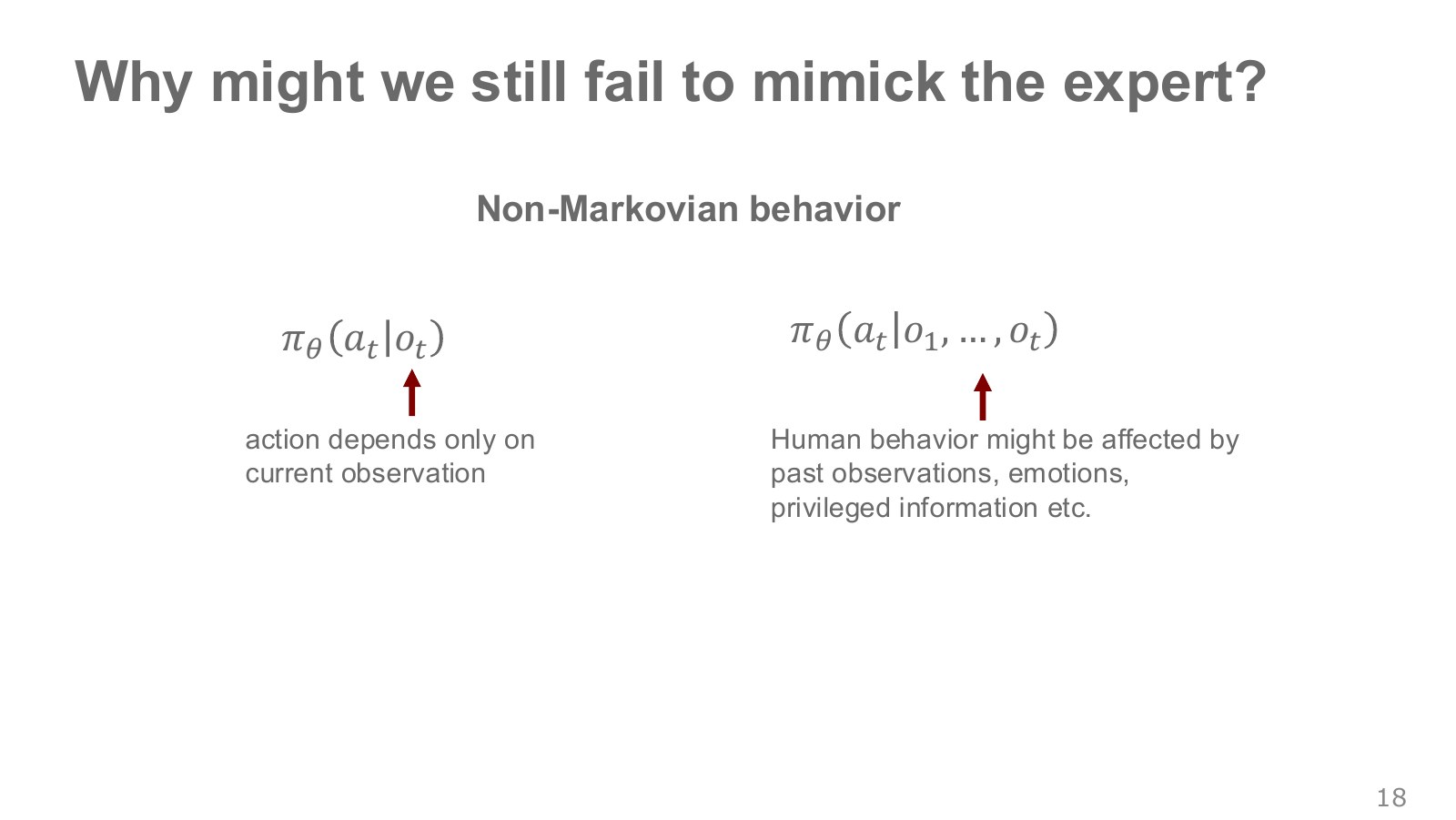
The demonstrator’s action is then not sufficiently described by a function of the current observation. Past views, intent or a recently checked blind spot may supply information unavailable to the policy. This is a problem of non-Markovian behavior relative to the current input.
Explore the symbols and calculation Distinguish policies using only current observations from policies conditioned on observation and action history
Read the equation in words
This contrasts a policy seeing only the present scene with one seeing past scenes and actions too. It is not an equality claiming identical computations.
Understand each symbol
- The action chosen at step : for example, a torque, a joint target or a movement direction, depending on the setup.
- The sensor observation at step . It is not assumed to equal the full physical state.
- A policy that maps an observation to an action distribution. The subscript denotes the weights that define it.
- Observation history from the beginning to the present.
- The history of actions executed before choosing the current action.
- Conditional notation: the information to the right of the bar is given. This is not a division sign.
Follow the calculation
- Consider which past information the current observation omits.
- If needed, add observations and earlier actions as time-ordered inputs.
Check with a small example
The same cup photograph may require different next actions depending on whether the gripper just closed or opened.
An illustrative example for understanding the equation.
denotes observation history from the beginning through the current step. Two actions at the same observation do not immediately establish human inconsistency: information used by the person may be missing from the policy input. Conversely, history may still leave different intentions or multiple valid approaches unexplained; those lead to the multimodal-distribution problem below. Original lecture, 25:28–27:31.
#P020 · Privileged observations: information visible to the demonstrator but not the robot
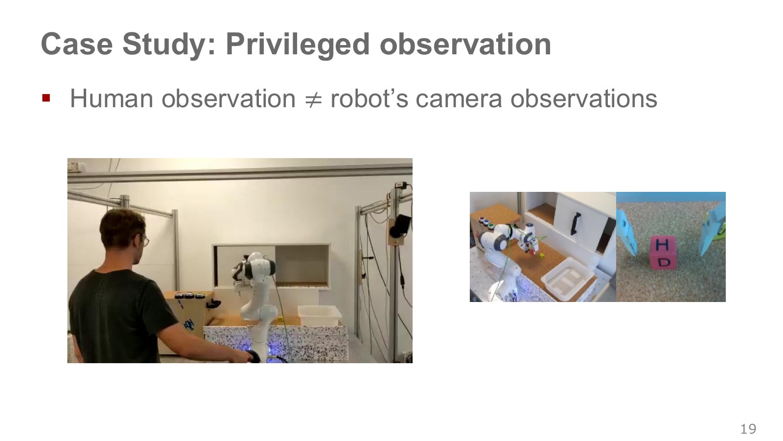
The person on the left can look around the robot and table directly. In the camera view on the right, an object may appear small or be hidden by the hand. A person may have checked a handle from another viewpoint while the policy must predict the same action without seeing it.
Such demonstrator-only information is called privileged information or a privileged observation. The term describes who has access to information, rather than one particular learning algorithm. A person demonstrating with exact object positions displayed by a simulator while the deployed policy receives only cameras is another example.
Options include having the demonstrator use the same camera view as the policy or providing the sensors the policy needs. Using training-only information requires a learning design that still works when it is unavailable at execution time. This is one reason more demonstrations alone cannot resolve every problem. Original lecture, 27:36–28:43.
#P021 · What can a history-aware model add?
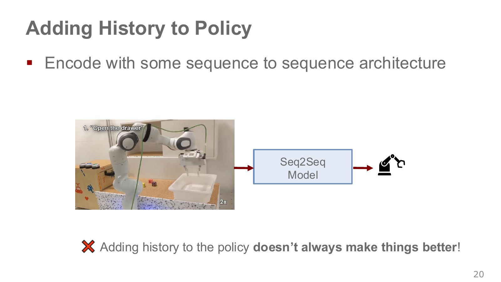
A sequence model computes relationships among ordered inputs. Encoding several past images and reading their sequence can reveal motion direction or recent-action context absent from one frame.
Seq2Seq in the figure means a structure mapping an input sequence to an output sequence or action. RNNs and LSTMs carry past information through internal state; Transformers allocate attention among inputs. Changing the architecture’s name does not automatically produce the needed memory. Input window, sampling interval, latency and computation also need specifying.
When past actions are inputs, inspect what fills those slots at execution time. Training with previous expert actions and executing with previous policy actions changes this input too. Adding memory and learning the right cues are separate challenges. Original lecture, 28:45–29:54 · Berkeley on history models, 8:59–9:46.
#P022 · Causal confusion: mistaking an outcome's trace for the reason to act
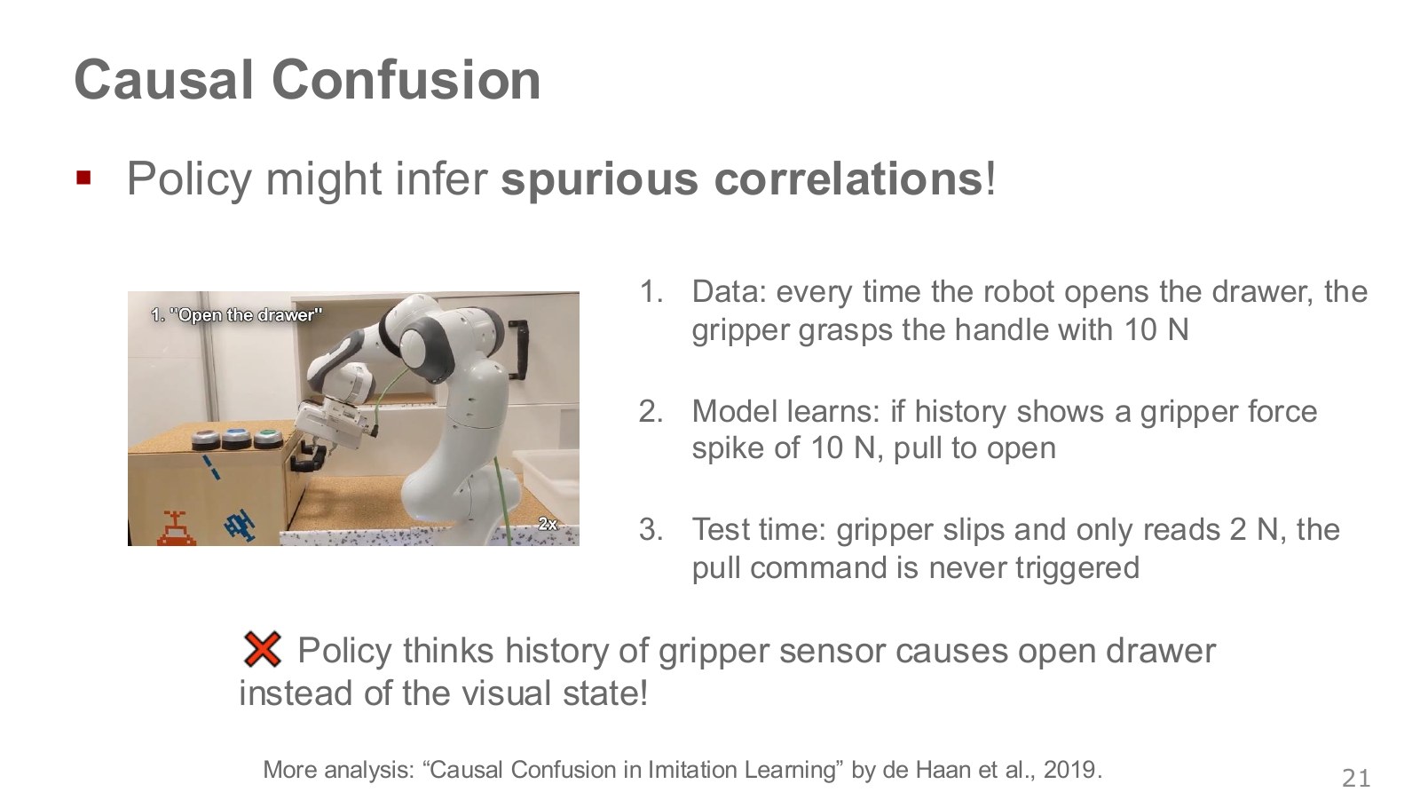
Suppose a gripper force sensor always reads 10 N before the demonstrator opens a drawer. A model might learn “pull when the signal is 10 N” instead of checking whether the handle is properly grasped. If the reading becomes 2 N at execution time, the pulling command may never appear.
When the force signal and handle contact always co-occur in training, the training loss alone may not distinguish which cue will remain useful under new conditions.
Correlation means two phenomena occur together in data. Causation concerns how a factor produces an outcome. A cue always accompanying an action in demonstrations need not remain a sound basis for acting after the environment changes. Policy learning studies this as causal confusion.
This does not make force sensors useless. Grasp state and force can be physically important. The issue is reliance on an incidental pairing between a particular number and an action while missing the contact or visual information required under changed conditions. The drawer is a conceptual example, not evidence against all force-based control.
Berkeley uses another example: a brake indicator. The driver sees a pedestrian and brakes, which switches on the indicator. A model predicting braking solely from that indicator can miss the moment when braking should begin. Longer history can provide more of these easy cues too. Berkeley, 9:58–12:38.
Masking cues or changing environmental conditions can probe what a model relies on. Merely enlarging it or supplying longer history does not guarantee causal understanding. Original lecture, 29:56–31:51 · de Haan et al.’s original paper and project.
#P023 · Multimodal actions: several ways to achieve one goal
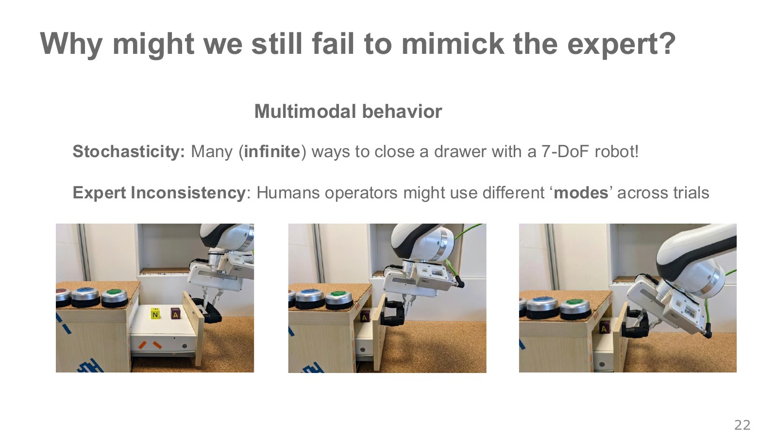
A drawer can be closed by grasping and pushing its handle or by pushing its front. The pictured arm can achieve the same goal through different approaches, from above or from the side. The redundancy discussed in Chapter 02 similarly allows different joint configurations for the same tool pose.
When separated actions frequently occur under similar inputs, the action distribution has several peaks. This is multimodality, or multiple modes. A mode here is a distinct way of acting, different from “multimodal” meaning several sensory types such as vision, language and force.
If different human approaches all succeed, none is necessarily a wrong target. The problem is how to represent that diversity when a policy is required to output one average value. Original lecture, 31:54–33:30.
#P024 · The average of two safe routes can head toward a tree
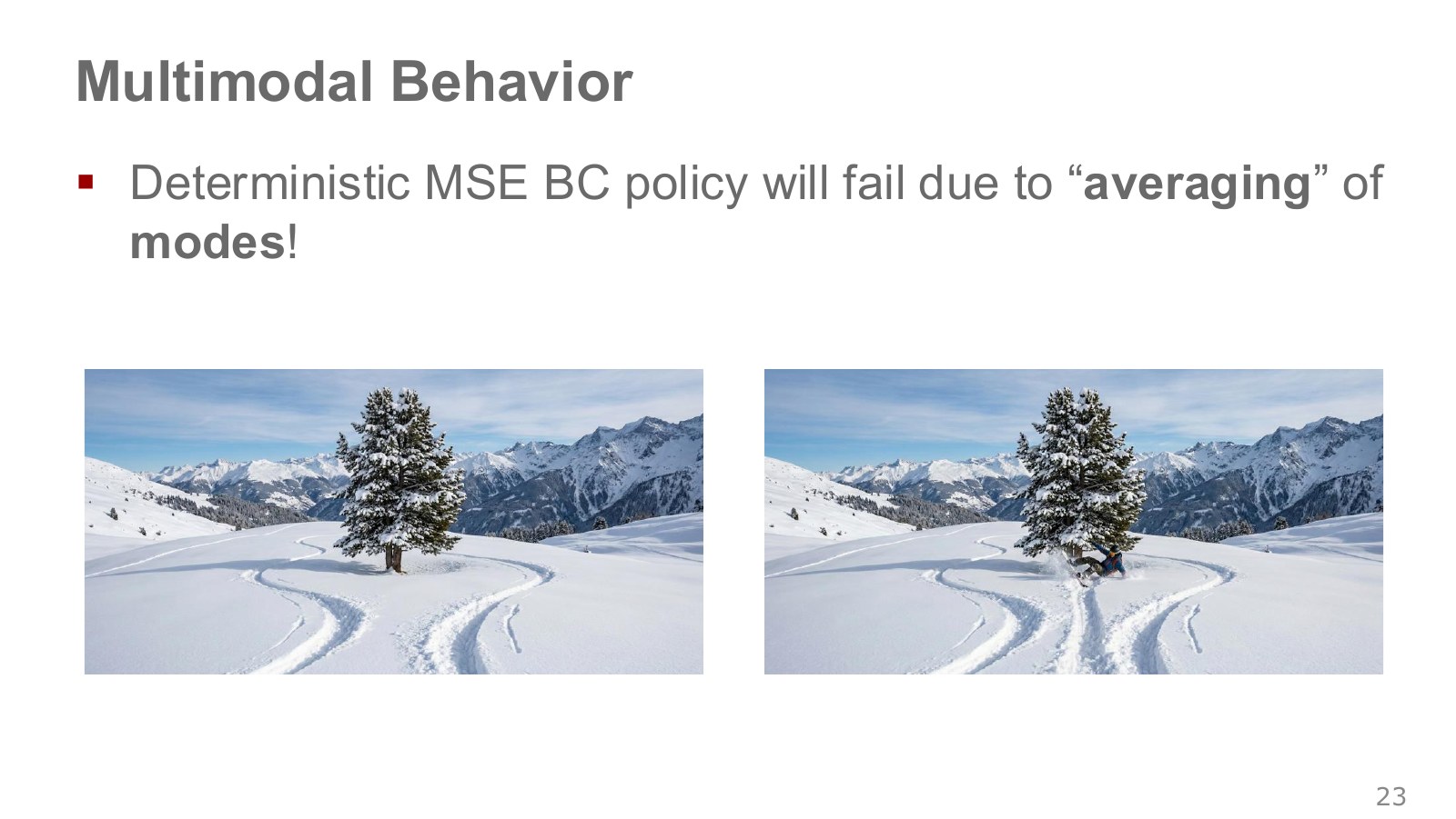
Tracks in snow pass a tree on both the left and the right. Their pointwise average can run between them, toward the tree. Averaging individually valid targets need not yield a good execution.
Suppose half the action targets for the same input are −1 and half +1. Minimizing squared error with one constant action gives the following.
Explore the symbols and calculation Equal-weight squared-error learning from opposite actions makes their mean, 0, the optimal single prediction
Read the equation in words
Fitting one number by squared error to opposite targets such as left and right selects their mean. Whether that mean is a good physical action is separate.
Understand each symbol
- The predicted action represented by one number.
- The prediction minimizing this loss.
Follow the calculation
- Square the difference from each target and add the two with equal one-half weights.
- Expanding leaves a squared term and a constant, so prediction 0 minimizes the square.
Check with a small example
Prediction 0 gives loss 1; prediction 1 gives loss 2. If the targets go around an obstacle on either side, their straight-ahead average can be dangerous.
An illustrative example for understanding the equation.
Under the error calculation, zero is optimal. But if −1 and +1 represent going around an obstacle on opposite sides, zero may provide no avoidance. MSE has not made an arithmetic mistake; predicting one point and representing multiple possible actions are different objectives.
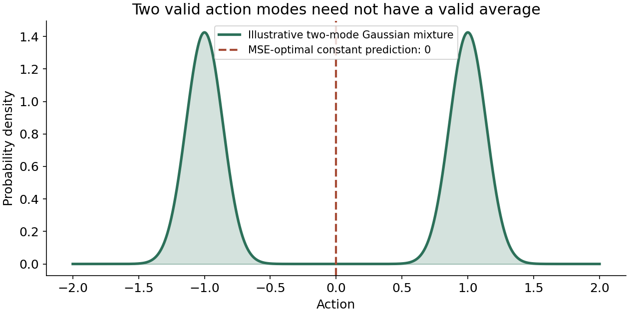
The vertical axis is probability density. Curve height is not the probability of one exact action; it describes concentration in nearby intervals. The optimal single prediction under squared loss is likewise related to a conditional mean. The tree analogy does not imply that averaging always causes collisions in every action representation. Examine the inputs, representation and arrangement of valid solutions together. Original lecture, 33:33–34:16.
#P025 · Gaussian mixtures: represent several action peaks instead of one mean
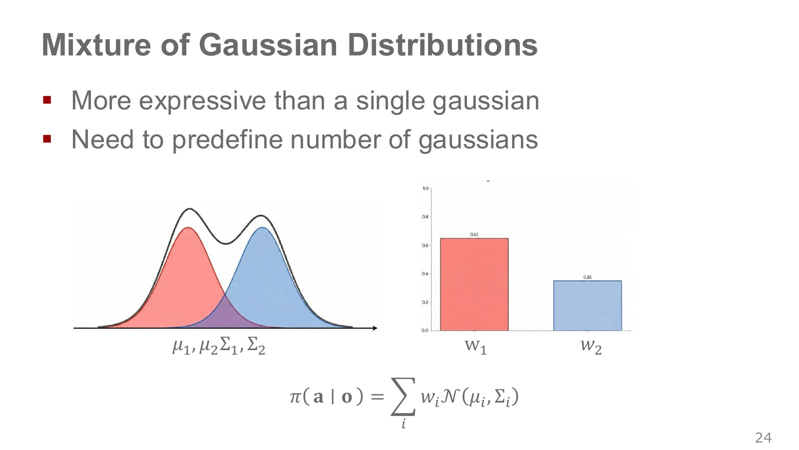
A Gaussian distribution is a bell-shaped distribution concentrated around a mean. Multiple action alternatives can be represented by a weighted sum of several Gaussians. The red and blue curves are individual components; the black curve is the combined distribution.
Explore the symbols and calculation Predict multiple means, covariances and mixing weights per observation to form a Gaussian-mixture action distribution
Read the equation in words
Mix several Gaussians to represent multiple peaks of possible actions instead of collapsing everything into one mean.
Understand each symbol
- A policy that maps an observation to an action distribution. The subscript denotes the weights that define it.
- The number of mixture components and their observation-dependent weights.
- Each Gaussian's mean action and covariance.
- The action density under a Gaussian with the given mean and covariance.
- Add every term over the indicated range, computing one term and repeating through the end of the range.
- Conditional notation: the information to the right of the bar is given. This is not a division sign.
Follow the calculation
- Predict each peak's mean, covariance and weight from the observation.
- Multiply each component's action density by its weight and sum. Weights must be nonnegative and sum to 1.
Check with a small example
Giving equal weight around −1 and +1 can assign high density to both ways around an obstacle instead of always selecting 0.
An illustrative example for understanding the equation.
is a component mean, is its covariance describing spread and joint variation among action components, and is its selection weight. Weights are nonnegative and sum to 1. The bars 0.65 and 0.35 give component proportions, not peak curve heights of 65% and 35%.
In a policy, these quantities are network outputs that change with the observation. To sample an action, first choose a component by its weight and then sample within it. Averaging the component means back into one final action can recreate the original averaging problem.
The number of components is usually fixed in advance, and outputting many means and covariances becomes burdensome in high-dimensional action spaces. Overlapping components also mean the visible peak count need not equal component count. A changed distribution representation requires a matching objective that increases demonstrated-action likelihood. Original lecture, 34:19–35:14 · Berkeley on mixture distributions.
Consider increasing mixture size from 10 to 1,000 components. In an illustrative seven-dimensional action model with diagonal-covariance Gaussians, each component needs seven means, seven standard deviations and one mixing-weight logit. That gives 150 outputs for ten components and 15,000 for 1,000. Standard deviations need a positive transformation, and weights need normalization to sum to 1. Free-parameter counts and covariance structure vary by implementation, but the example shows why adding components alone does not make complex action distributions easy to learn. This motivates the conditional latent-variable models below.
#P026 · Autoregressive discretization: choose action coordinates conditionally, one at a time
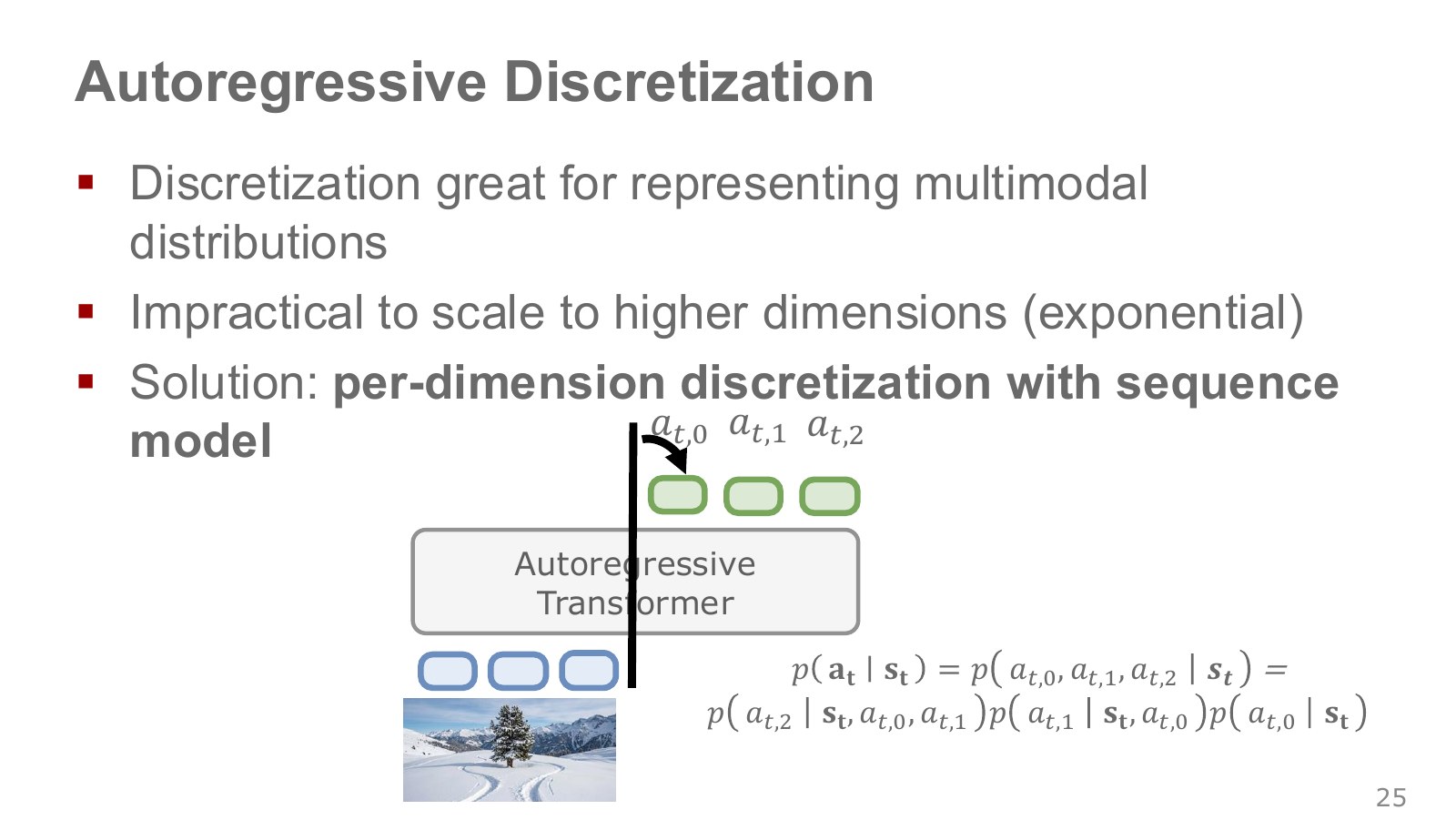
Dividing continuous steering into intervals called bins lets a classifier output selection probabilities for them. Assigning high probability to left and right bins and low probability to the center can represent several modes.
The challenge is multidimensional actions. Dividing each coordinate into bins and classifying every combination of coordinates at once creates choices. Seven coordinates with 100 bins each give combinations.
An autoregressive model chooses each action component conditioned on earlier selected components. By the probability chain rule, a three-component action can be written as follows.
Explore the symbols and calculation Generate components of one action vector sequentially, conditioning each on components already selected
Read the equation in words
Choose the components of one action vector in sequence, letting later components depend on earlier choices. This order differs from acting over physical time.
Understand each symbol
- The state at step , containing information such as position and velocity needed to predict what happens next.
- Three different components of the action vector at the same step .
- Conditional notation: the information to the right of the bar is given. This is not a division sign.
Follow the calculation
- Compute the probability of the first action component.
- Condition on that choice to compute the second and third components, then multiply their probabilities.
Check with a small example
Conditional probabilities 0.5, 0.4 and 0.8 give combination probability .
An illustrative example for understanding the equation.
index three coordinates of one action vector at the same time step, not three time steps. Selecting a later direction consistent with an earlier direction can represent coherent combinations more easily than sampling coordinates independently.
The return arrow feeds a generated token into the next prediction. Each component’s output list can have entries, but generation is sequential, and the model’s computational cost is not guaranteed to be simply . Coordinate order, quantization precision and execution latency matter too. A Transformer is one available sequence model; a large language model is not mandatory. Original lecture, 35:16–37:24.
#P027 · Diffusion models: generate condition-dependent actions from noise
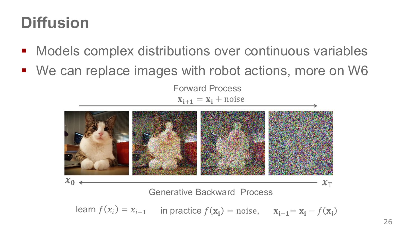
The cat image becomes noisier toward the right. The forward process adds noise to clean data to construct training inputs; reverse generation starts from noise and progressively recovers structure.
Keep diffusion indices separate from time steps when the robot physically acts. Here, let actual control time be and noise-step index be . A common expression for constructing a noisy training sample is:
Explore the symbols and calculation Diffusion training mixes clean samples and Gaussian noise at step-dependent ratios to construct inputs
Read the equation in words
Mix clean action data and Gaussian noise at specified ratios to create diffusion-training inputs. Noise steps differ from the robot's physical time.
Understand each symbol
- Sample a Gaussian noise vector with component means 0 and variances 1.
- A clean action sample and its sample at noise step .
- The cumulative coefficient for retained original signal. The two mixing coefficients themselves need not sum to 1.
Follow the calculation
- Choose the cumulative proportion of signal to retain.
- Multiply data and noise by the square roots of their respective proportions and add.
Check with a small example
Retained proportion 0.64 gives data coefficient 0.8 and noise coefficient 0.6. Clean value 1 and noise 0.5 then produce input 1.1.
An illustrative example for understanding the equation.
is clean data, sampled noise, and sets the signal proportion retained at that step. A model can learn to predict the added noise, for example, given the noise step and current observation. Actual reverse updates include schedules and coefficients, so the original phrase “subtract the noise” is a shorthand for the principle.
In robotics, the generated object can be an action vector or short action sequence instead of a picture, conditioned on the current camera observation and goal. Several denoising computations for one action do not mean the robot physically moves at every computation step.
The original Diffusion Policy project connects observation-conditioned action-sequence generation with real robot tasks and replanning after executing a short segment. It considers both multiple modes and consistent execution of a selected approach. These notes do not report training that model; diffusion training is developed further in the later generative-model chapter. Original lecture, 37:28–39:06.
#P028 · Latent variables: specifying alternative ways to act in the same scene
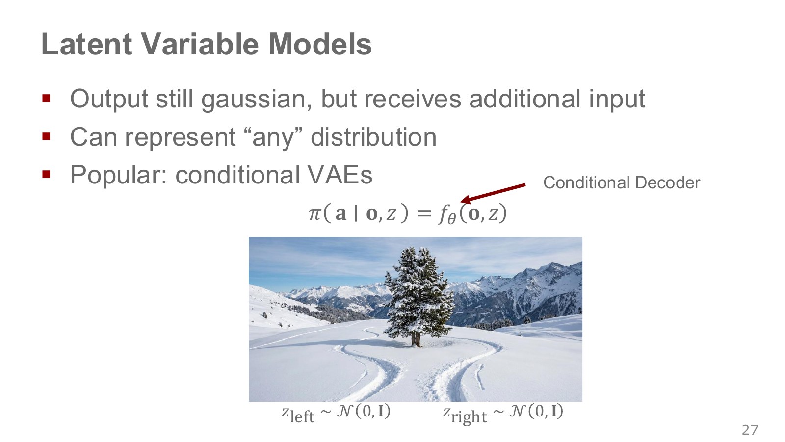
A latent variable is an internal variable learned to explain behavioral differences without a direct target name in the data. In the same scene before a tree, one might produce a leftward route and another a rightward route.
A decoder is a network mapping observations and latent variables to an action distribution. Adding input conditions makes it a conditional decoder.
Explore the symbols and calculation A conditional decoder uses a latent execution mode to output an observation-conditioned action distribution
Read the equation in words
Different latent values can produce different approaches under the same observation. Sample a latent value first, then use it to generate actions.
Understand each symbol
- A latent vector representing factors such as execution style that the model does not directly observe. It is sampled or inferred by an encoder.
- The prior distribution of latent values before observing the data.
- The sensor observation at step . It is not assumed to equal the full physical state.
- The parameters collecting the trainable weights of the network or policy.
- Conditional notation: the information to the right of the bar is given. This is not a division sign.
Follow the calculation
- Sample a latent vector from the prior.
- Feed the observation and latent vector together into the decoder to obtain an action distribution.
Check with a small example
For the same cup, latent values can represent approaches from the left or right. Their actual meaning must be learned from data.
An illustrative example for understanding the equation.
We can use a simple prior such as . Even if the output distribution is simple at a fixed , combining outcomes across different can represent a complex distribution. The capacity of a sufficiently expressive model and successful training of that model are separate matters.
Adding arbitrary noise to a network does not automatically create left and right modes. A network may ignore random inputs unrelated to target actions. The conditional variational autoencoder (CVAE) below also builds a training path that infers useful from demonstrations. Original lecture, 39:11–40:17.
#P029 · Task conditions specify the goal; latent variables specify how to perform it
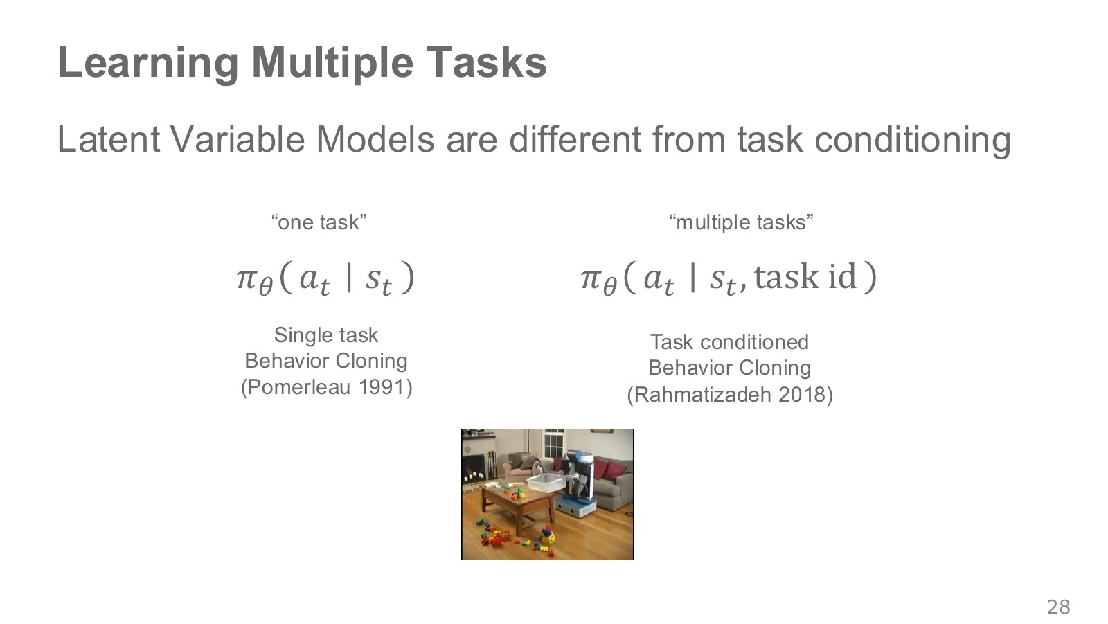
“Open the drawer” and “close the drawer” differ in which goal to pursue. Grasping it from above or from the side differs in how to pursue the same goal. Separating task conditions from latent action modes reduces confusion.
A policy using a task ID can be written as . Representing three tasks by vectors [1,0,0], [0,1,0] and [0,0,1] is one-hot encoding. Language or a goal image can also specify the task.
Adding a task condition need not leave only one way to achieve it. We can therefore condition on both goal and execution mode as . Changing the goal and representing diverse executions within it are different problems. Original lecture, 40:22–41:01.
#P030 · Has the task succeeded if the door moved halfway?
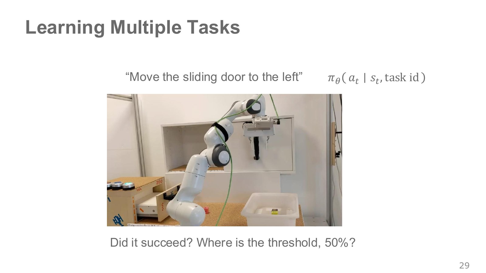
Suppose the instruction only says “move the sliding door left.” One person might consider a halfway movement sufficient, while another expects it to move all the way. The 50% in the photograph is not policy confidence; it asks how far the door must move to count as success.
A single task name such as “open” can obscure the desired displacement and end state of a continuously moving object. Evaluation must specify target position, tolerance and any required states of other objects. Supplying a target image or state is one starting point for expressing continuous goals. Original lecture, 41:03–42:47.
#P031 · Policies conditioned on a goal state
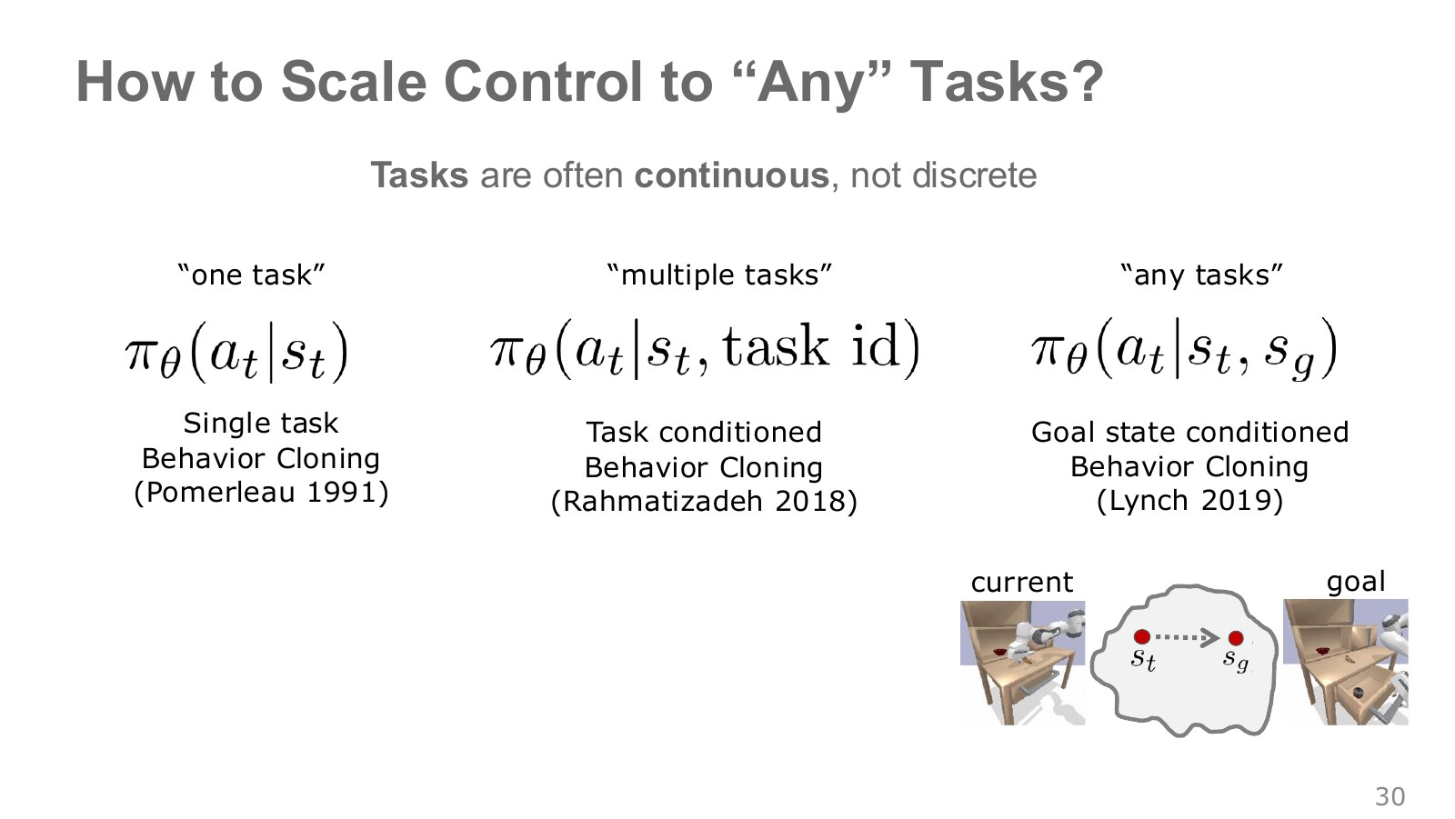
Instead of assigning a new task number to every door-opening distance or location, supply the desired end state . A goal-conditioned policy acts toward that target from current state .
Explore the symbols and calculation A goal-conditioned policy takes current and desired goal states and forms a next-action distribution
Read the equation in words
Give the policy a desired destination alongside current state. Different goals can lead to different actions from the same state.
Understand each symbol
- The state at step , containing information such as position and velocity needed to predict what happens next.
- The action chosen at step : for example, a torque, a joint target or a movement direction, depending on the setup.
- The parameters collecting the trainable weights of the network or policy.
- The desired goal state, distinct from the current state.
- Conditional notation: the information to the right of the bar is given. This is not a division sign.
Follow the calculation
- Supply current and goal states as distinct inputs.
- Compute the next-action distribution appropriate to that goal.
Check with a small example
From the center of a table, a policy can learn to approach left for the left cup and right for the right cup.
An illustrative example for understanding the equation.
The policy learns actions connecting the current and target scenes on the right. From the same starting scene, a different target door position should require different actions. Goal meaning and sensor representation must also match between training and execution.
Berkeley describes training by relabeling each recorded trip to a destination with its final state as the goal. This can cover more states than records for one destination alone. It does not guarantee solving unseen start–goal combinations or physically impossible goals. Berkeley on goal relabeling, 0:24–3:10 · Original lecture, 42:50–43:15.
#P033 · Play data is not random motor commands
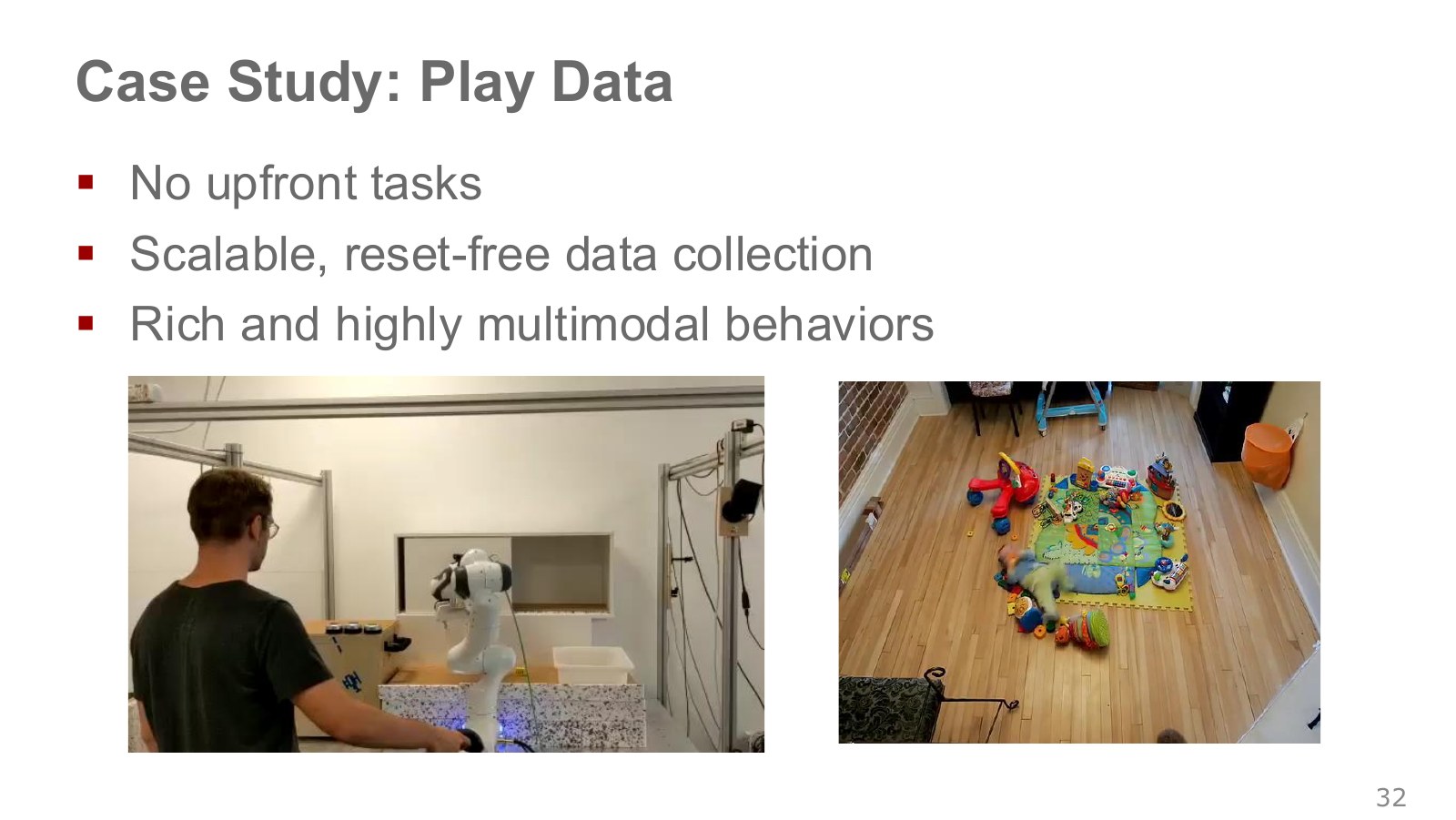
Play data records a person continuously teleoperating a robot through diverse interactions, such as opening, closing and moving objects. Collection can continue without preassigning a task name to every episode or resetting to the same initial scene each time.
Like the pictured toy play, it explores possibilities instead of repeating one prescribed sequence. But a person collects these records; they do not show a robot autonomously learning curiosity. The movements are also structured by human understanding of object use, unlike random torques.
Opening and closing a door, or correcting a failed grasp, can record transitions between tasks and recovery behavior. Diversity does not establish complete coverage, so inspect which objects, contacts and views were actually collected. Original lecture, 43:17–44:19 · Original Learning Latent Plans from Play paper.
#P034 · Sampling short windows from long play records
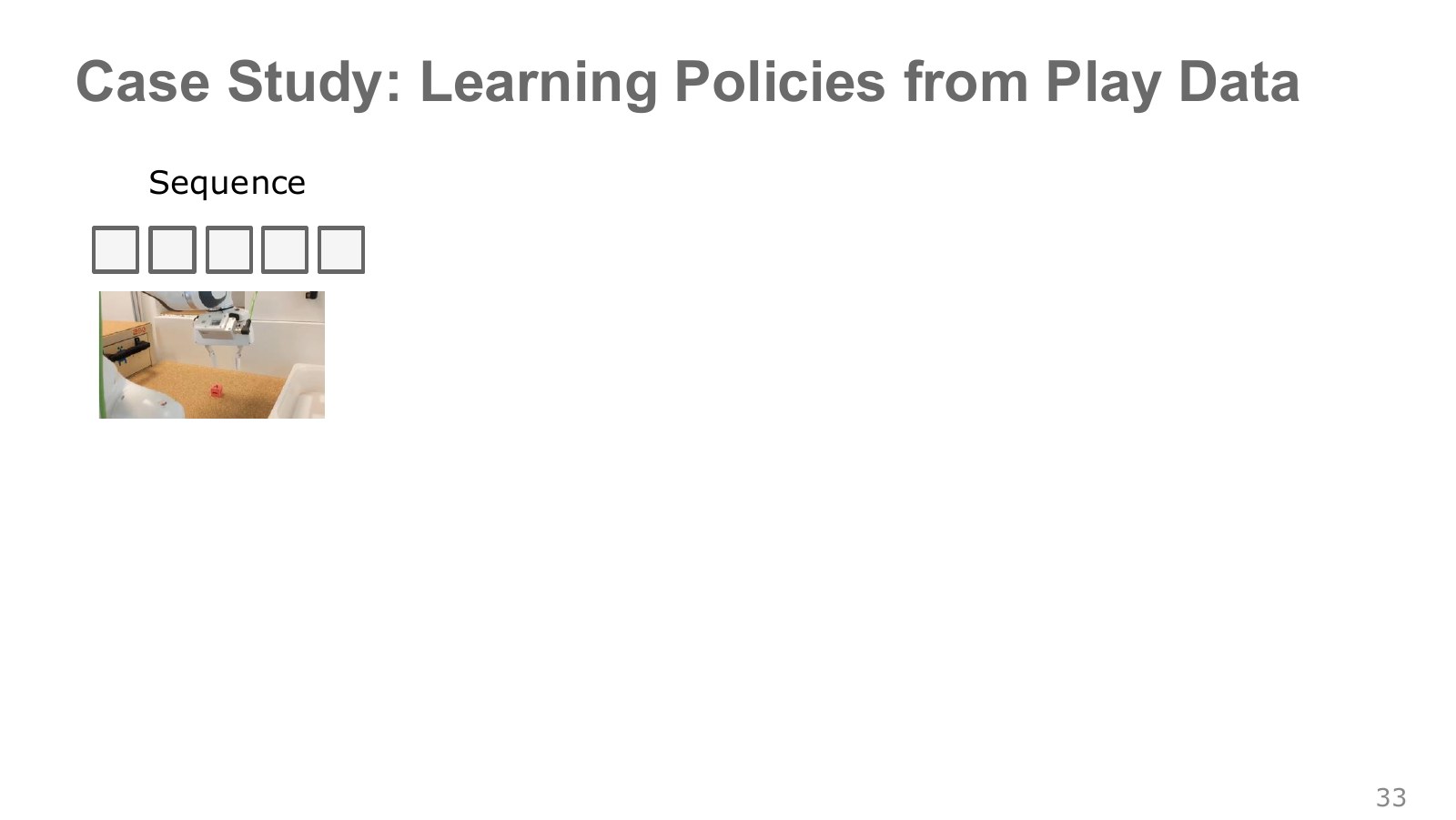
The boxes above represent consecutive observations. Sampling a short time window from a long record also selects the actions actually performed between them. Sampling a window means choosing the start and end of a consecutive segment, not shuffling its order.
For example, select observations and intervening actions as one segment. The last observation is the scene those actions actually reached. The record can then supply an example of actions leading to that final scene.
Sampling isolated frames makes it difficult to identify consistent execution across a whole segment. The plan recognizer below reads the complete segment to infer how that endpoint was reached. Original lecture, 44:22–44:56.
#P035 · Self-supervised learning by relabeling the final scene as a goal
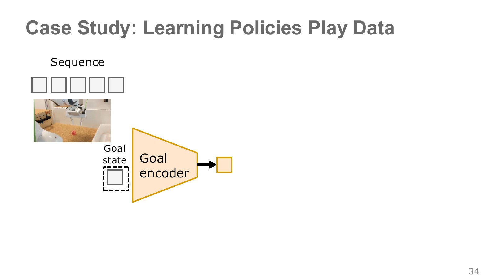
The yellow triangular goal encoder converts the final scene into a feature vector a network can use. An encoder maps useful input information into another representation; it is not simply classifying every pixel into one task name.
Earlier scenes become current inputs, the last scene becomes the goal, and recorded actions become targets. This is goal relabeling: constructing goal targets from records without separate human task labels. Because the data itself supplies the learning signal, it is called self-supervised learning.
“Self” here refers to constructing goal labels, not to collecting observation–action records without people. Inputs written as in the paper can also be encoded visual and proprioceptive features. They should not automatically be equated with Chapter 02’s full physical state.
Multiple paths can connect the same start and end, so adding the goal does not resolve every multimodality issue. The next block represents the execution style between them separately. Original paper, pp. 4–5.
#P036 · Plan recognition and plan proposal see different information
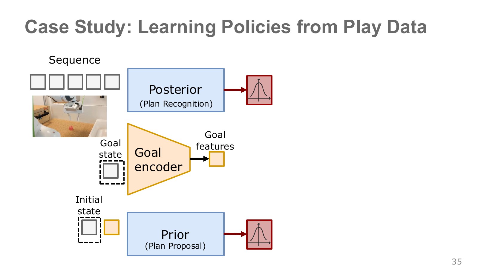
The upper plan-recognition path reads the whole segment during training. Seeing how the object was approached, grasped and moved lets it form a distribution over latent plans explaining the behavior. The original labels this path posterior.
The lower plan-proposal path sees only the starting and goal states. Without knowing the actual intermediate route, it must propose a distribution of plans that could connect them. This is the original’s prior path.
A prior assigns a distribution over plans before seeing the particular demonstration’s intermediate actions; a posterior infers plans using that observed segment. The trained plan-recognition network approximates a true posterior that is difficult to calculate directly.
At execution time, the correct future demonstration segment is unavailable. This is why both paths are needed: use whole-segment information available during training, but connect it to plan proposal from start and goal during execution. Original lecture, 45:00–45:46.
#P037 · The KL term connects training-time and execution-time plans
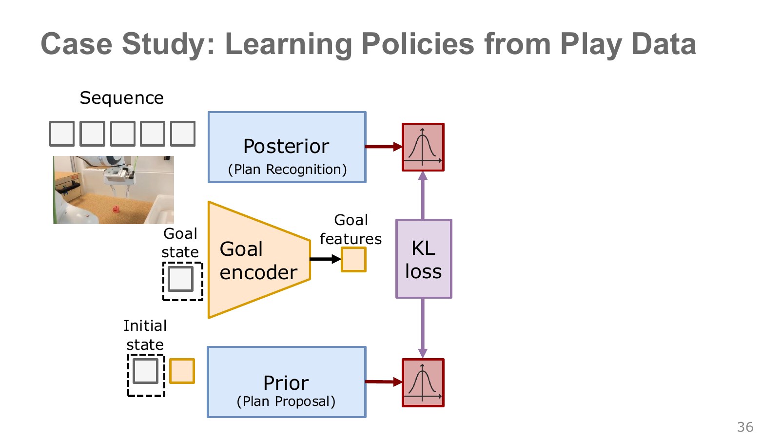
The purple KL-loss box compares the two plan distributions. Kullback–Leibler (KL) divergence measures how differently one distribution accounts for values frequently produced by another. It is zero for identical distributions and generally changes when their order is reversed, unlike an ordinary symmetric distance.
Training encourages the execution-time proposal to assign likelihood to plans identified from demonstrations. If recognition uses codes the proposal almost never samples, a decoder that works during training may become useless in execution.
Matching distributions is not sufficient by itself. Both could output the same uninformative distribution and achieve low KL loss. The next page therefore optimizes it together with action reconstruction. Check whether actually helps explain behavioral differences. Original lecture, 45:48–46:03.
#P038 · Reconstructing actions from current observations, goals and a latent plan
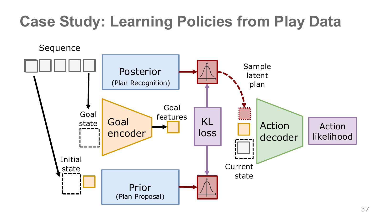
The green action decoder receives current-state features, goal features and a sampled latent plan to explain demonstrated actions. Sampling selects one value permitted by a distribution according to its probability or density.
During training, the decoder uses inferred by recognition from the full demonstration and reconstructs its actions with high likelihood. The action-likelihood box evaluates how well the predicted distribution explains the actual actions. The policy’s central reconstruction target is demonstrated behavior, rather than the pixels of an image.
During execution, recognition is removed and the proposal supplies from start and goal. The decoder still receives freshly observed state at every action, so fixing a latent plan differs from blindly replaying a fixed sequence of motor commands.
In the original paper’s diagram, training is on the left and execution on the right. Notice first that the “entire sequence” input disappears on the right.
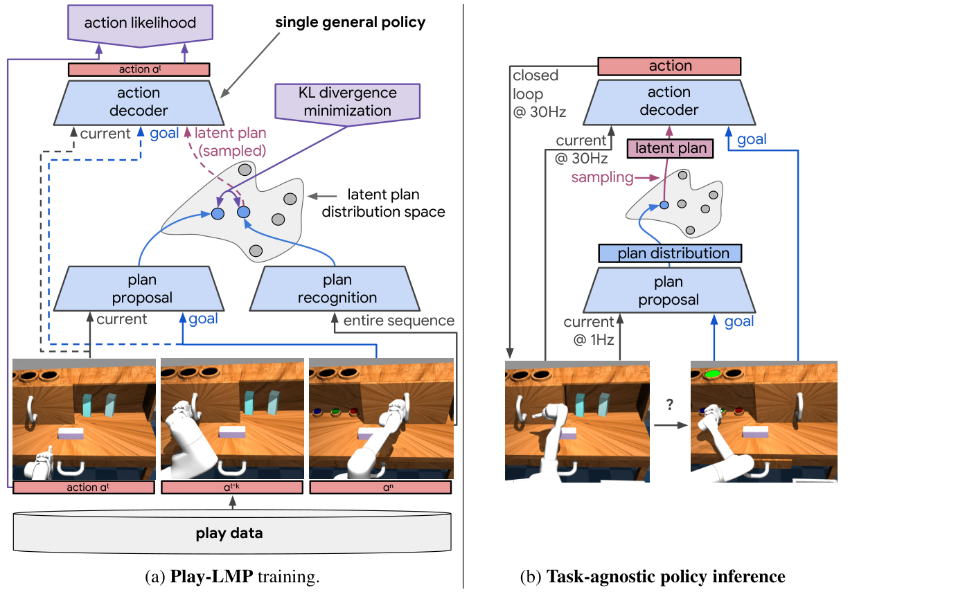
The 1 Hz plan proposal and 30 Hz action computation belong to that study’s timing structure. They illustrate a hierarchy with slower planning and faster responses to current state. Latent-plan models need not all use those rates. Original paper, pp. 2 and 5–6 · Original lecture, 46:05–46:39.
#P039 · Connecting target images and language to a shared goal representation
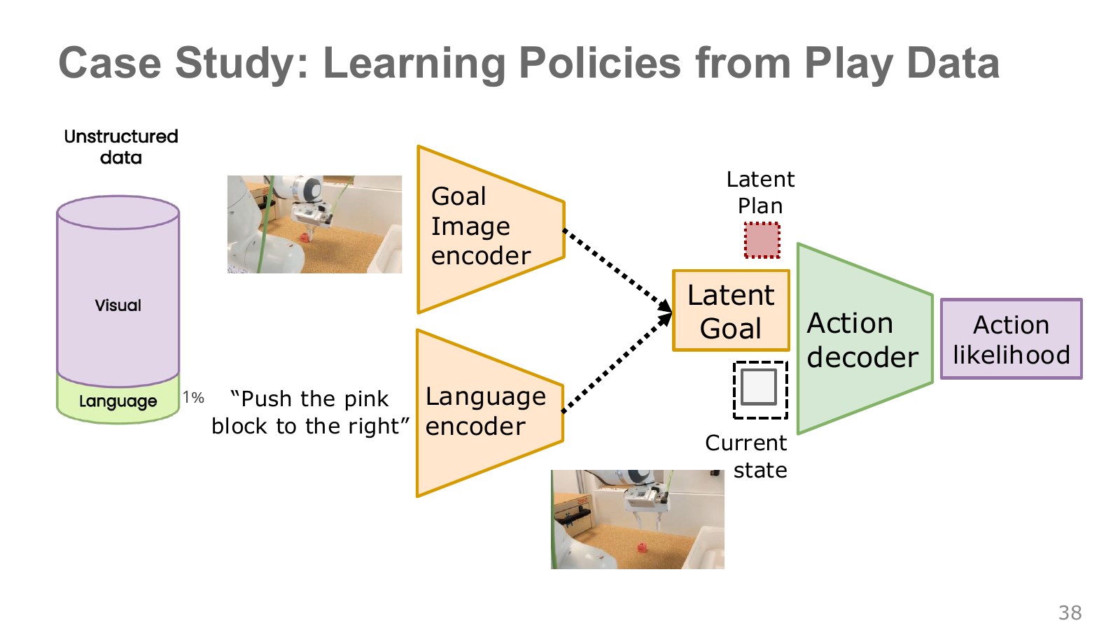
Earlier, the goal was an image of a desired final scene. A person may instead want to say “push the pink block to the right.” The two yellow encoders map goal images and language sentences into goal features the policy can use.
People need not annotate every segment of free-form manipulation with language. Many segments teach control using their final image as the goal; descriptions attached to a subset connect language with goal representations. Which sentence labels which segment still matters for language-driven execution. Language-conditioned imitation learning paper
Learning to align the two representations lets the method combine many image-goal play segments with a smaller language-labeled subset. The small language fraction in the figure represents partial language labeling in that study, not a rule that the same proportion suffices for every task.
A shared representation does not automatically turn every sentence into the desired scene. There must be evidence connecting the named object and direction to the actual view. As with the ambiguous “blue one,” an unclear goal can still require confirmation.
Distinguish a latent goal from a latent plan: goal features specify what to achieve, while plan features specify how to connect the current situation to that goal. Original lecture, 46:41–47:18 · Follow-up work on language-conditioned learning from play.
#P040 · Optimizing a lower bound when likelihood is hard to compute directly
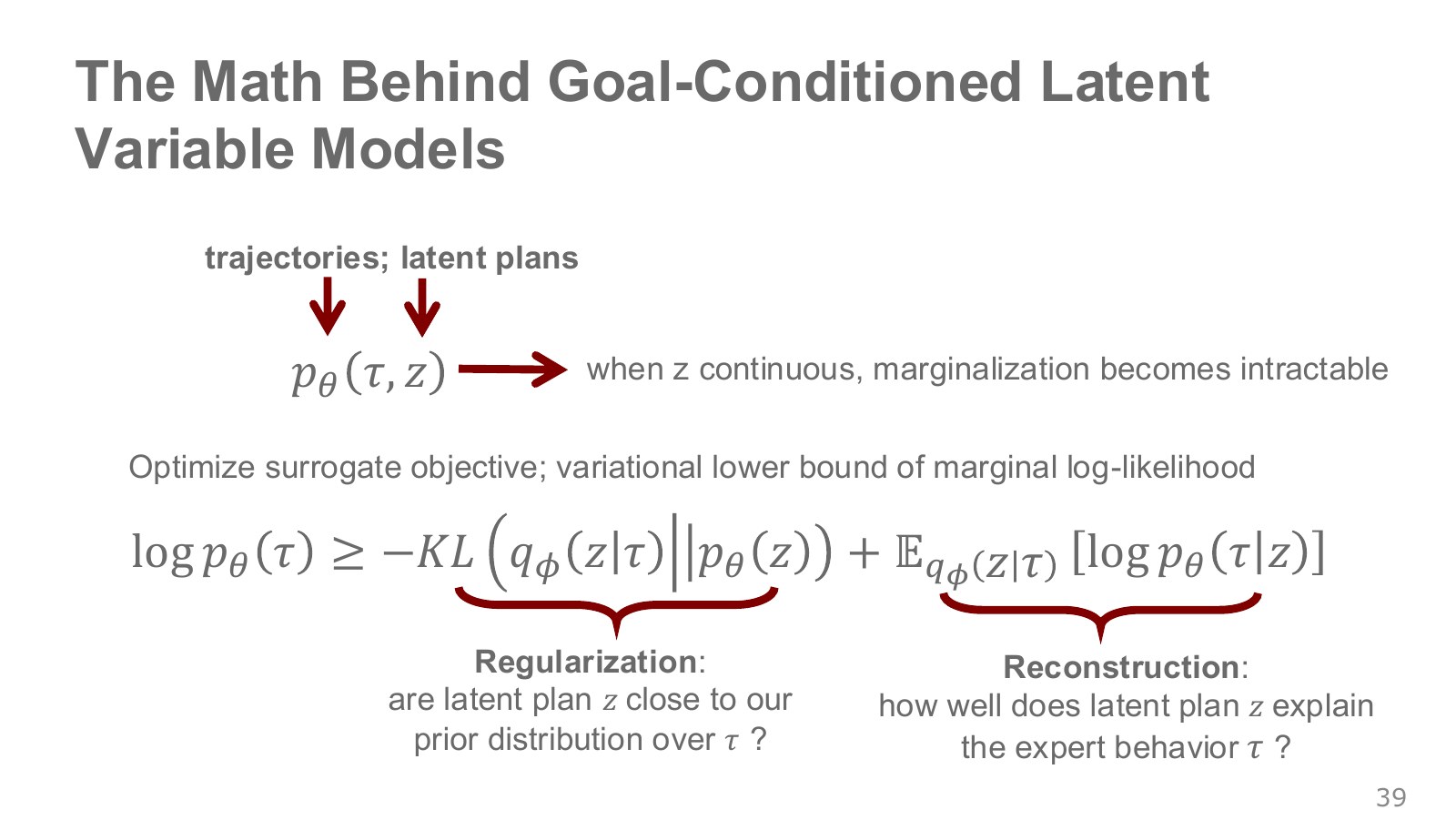
Several latent plans can explain the same demonstration. Without knowing , computing its likelihood requires combining, for every plan, the plan’s likelihood with the likelihood of the demonstration under it. Continuous latent variables require an integral in place of a sum.
Explore the symbols and calculation Marginal demonstration likelihood integrates plan-conditioned likelihood weighted by the plan prior
Read the equation in words
Combine all latent plans that could generate a demonstration to obtain its overall likelihood. Continuous latent values require integration instead of summation.
Understand each symbol
- One trajectory containing states and actions in time order. This symbol does not denote an angle.
- A latent vector representing factors such as execution style that the model does not directly observe. It is sampled or inferred by an encoder.
- The demonstration likelihood given a plan.
- The prior over latent plans.
- A weighted sum over the entire continuous latent space.
- Conditional notation: the information to the right of the bar is given. This is not a division sign.
Follow the calculation
- Compute demonstration likelihood for each latent plan.
- Weight it by that plan's prior probability or density and combine across plans.
Check with a small example
Two discrete plans with probabilities 0.6 and 0.4 and demonstration likelihoods 0.5 and 0.2 give marginal likelihood .
An illustrative example for understanding the equation.
Summing out a hidden variable this way is marginalization. Continuous variables are not always intractable in themselves. The difficulty here is accurately and efficiently evaluating an integral involving a complex neural-network decoder.
In this section, is shorthand for the demonstration segment being learned. The actual action decoder conditions each action likelihood on the corresponding observation within that segment. The expression should not be read as a world model generating all physical state transitions.
Introducing a distribution that infers useful plans from a demonstration lets us optimize a variational lower bound, the ELBO, on log-likelihood.
Explore the symbols and calculation The ELBO is a log-likelihood lower bound: expected reconstruction log-likelihood minus KL between approximate posterior and prior
Read the equation in words
Build a lower objective for a demonstration log-likelihood that is difficult to compute directly. Increase explanatory fit while discouraging excessive divergence of the encoder distribution from the prior.
Understand each symbol
- One trajectory containing states and actions in time order. This symbol does not denote an angle.
- A latent vector representing factors such as execution style that the model does not directly observe. It is sampled or inferred by an encoder.
- The parameters collecting the trainable weights of the network or policy.
- Weights of a different network. Read which model they belong to together with the calculation steps.
- KL divergence comparing two distributions. It is nonnegative and generally changes when the direction is reversed.
- The approximate posterior inferring a demonstration's latent plan from its whole sequence.
- Here this is a log-likelihood lower bound to maximize, rather than a loss to minimize.
- An expectation: an average over possible outcomes weighted by their probabilities.
- The natural logarithm. It converts products into sums and is defined only for positive inputs.
- Conditional notation: the information to the right of the bar is given. This is not a division sign.
Follow the calculation
- Average reconstruction log-likelihood under the encoder's inferred latent distribution.
- Subtract its KL divergence from the prior and maximize the resulting bound.
Check with a small example
Expected reconstruction −2 and KL 0.5 give lower bound −2.5. The next identity relates improvement of the bound to actual log-likelihood through a posterior-KL gap.
An illustrative example for understanding the equation.
are the generative model’s weights, and the weights of the model inferring plans from demonstrations. denotes an average under the distribution, not just one sampled value of . Sampling can estimate this average and its gradients in practice.
The first term is reconstruction: it increases when demonstration-inferred plans explain the actual actions well. The second is regularization, penalizing divergence from the prior used for execution. Training maximizes the whole expression or minimizes its negative as a loss.
The crucial symbol is . We should not unconditionally replace it with equality to the exact log-likelihood. The gap relates to the difference between approximate and true posterior distributions. Original lecture, 47:22–48:41 · Berkeley variational-inference slides, pp. 11–16 · Kingma and Welling’s original VAE paper.
#P041 · Mapping conditional-ELBO notation to the three networks
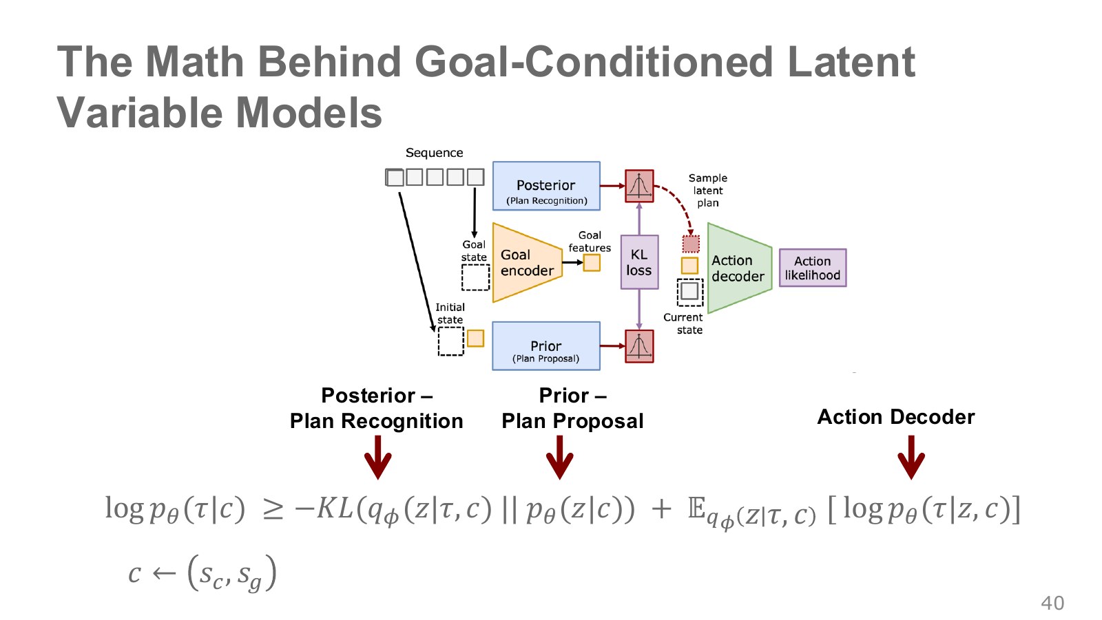
With a goal condition, let contain start and goal information. The same expression gains condition . Identify where posterior, prior and action decoder enter the original diagram.
Explore the symbols and calculation The goal-conditioned ELBO jointly trains whole-demonstration recognition, start-and-goal proposal and the action decoder
Read the equation in words
A latent-plan bound with conditions such as start and goal known. Distinguish execution-time conditions from the full demonstration available only during training.
Understand each symbol
- One trajectory containing states and actions in time order. This symbol does not denote an angle.
- A latent vector representing factors such as execution style that the model does not directly observe. It is sampled or inferred by an encoder.
- The parameters collecting the trainable weights of the network or policy.
- Weights of a different network. Read which model they belong to together with the calculation steps.
- KL divergence comparing two distributions. It is nonnegative and generally changes when the direction is reversed.
- Conditions available during execution, such as start and goal.
- A distribution inferring plans from the full demonstration and conditions.
- The plan prior obtained from conditions alone during execution.
- An expectation: an average over possible outcomes weighted by their probabilities.
- The natural logarithm. It converts products into sums and is defined only for positive inputs.
- Conditional notation: the information to the right of the bar is given. This is not a division sign.
Follow the calculation
- During training, infer plans using an encoder that sees conditions and demonstrations together.
- Subtract from reconstruction the KL to the plan prior predicted using only execution-time conditions.
Check with a small example
With starting position and target cup as conditions, future demonstration actions are unavailable during execution. The conditional prior must propose an appropriate plan.
An illustrative example for understanding the equation.
| Expression | Diagram block | Available information |
|---|---|---|
| Plan recognition; approximate posterior | Full demonstration segment plus start and goal during training | |
| Plan proposal; conditional prior | Start and goal; also available during execution | |
| Demonstration likelihood under the action decoder | Plan, goal and each step’s observation explain demonstrated actions. |
Because the true posterior is difficult to compute exactly, network approximates it. For the same latent variable, the distribution before seeing the full demonstration and the inferred distribution after seeing it have different roles.
The following identity shows why this is a lower bound.
Explore the symbols and calculation The gap between exact log-likelihood and ELBO is the nonnegative KL between approximate and true posteriors
Read the equation in words
The gap is the KL divergence from approximate to true posterior. Its nonnegativity makes the ELBO a lower bound.
Understand each symbol
- One trajectory containing states and actions in time order. This symbol does not denote an angle.
- A latent vector representing factors such as execution style that the model does not directly observe. It is sampled or inferred by an encoder.
- KL divergence comparing two distributions. It is nonnegative and generally changes when the direction is reversed.
- The true posterior after observing demonstration and conditions, distinct from the execution-time prior.
- The encoder's approximate posterior.
- The natural logarithm. It converts products into sums and is defined only for positive inputs.
- Conditional notation: the information to the right of the bar is given. This is not a division sign.
Follow the calculation
- A difference between true and approximate posteriors leaves a gap.
- When the distributions match, KL is zero and the bound equals the exact value.
Check with a small example
Log-likelihood −2 and lower bound −2.7 give a KL gap of 0.7. Using a lower bound alone does not guarantee exact posterior inference.
An illustrative example for understanding the equation.
The right side differs from the earlier regularizer. That term compares with the prior; this identity compares with the true posterior. Similar notation should not obscure the different comparisons.
I checked this identity with a small two-plan calculation. Prior probabilities 0.6 and 0.4 and data likelihoods 0.8 and 0.2 give marginal likelihood 0.56. With an arbitrary approximate posterior 0.7 and 0.3, log marginal likelihood is about −0.5798 and ELBO −0.6606, leaving a nonnegative gap of 0.0808. Matching the approximate to the true posterior makes the gap zero. This is a conceptual discrete latent-variable example, not a trained CVAE result.
The objectives connect reconstructing plans inferred from whole demonstrations during training with proposing corresponding plans from start and goal at execution. Their success must be evaluated through actual goal reaching and recovery as well as the objective value. Original lecture, 48:45–49:21 · Play-LMP’s three components, original paper pp. 5–6.
#P042 · Related studies develop different parts of the problem
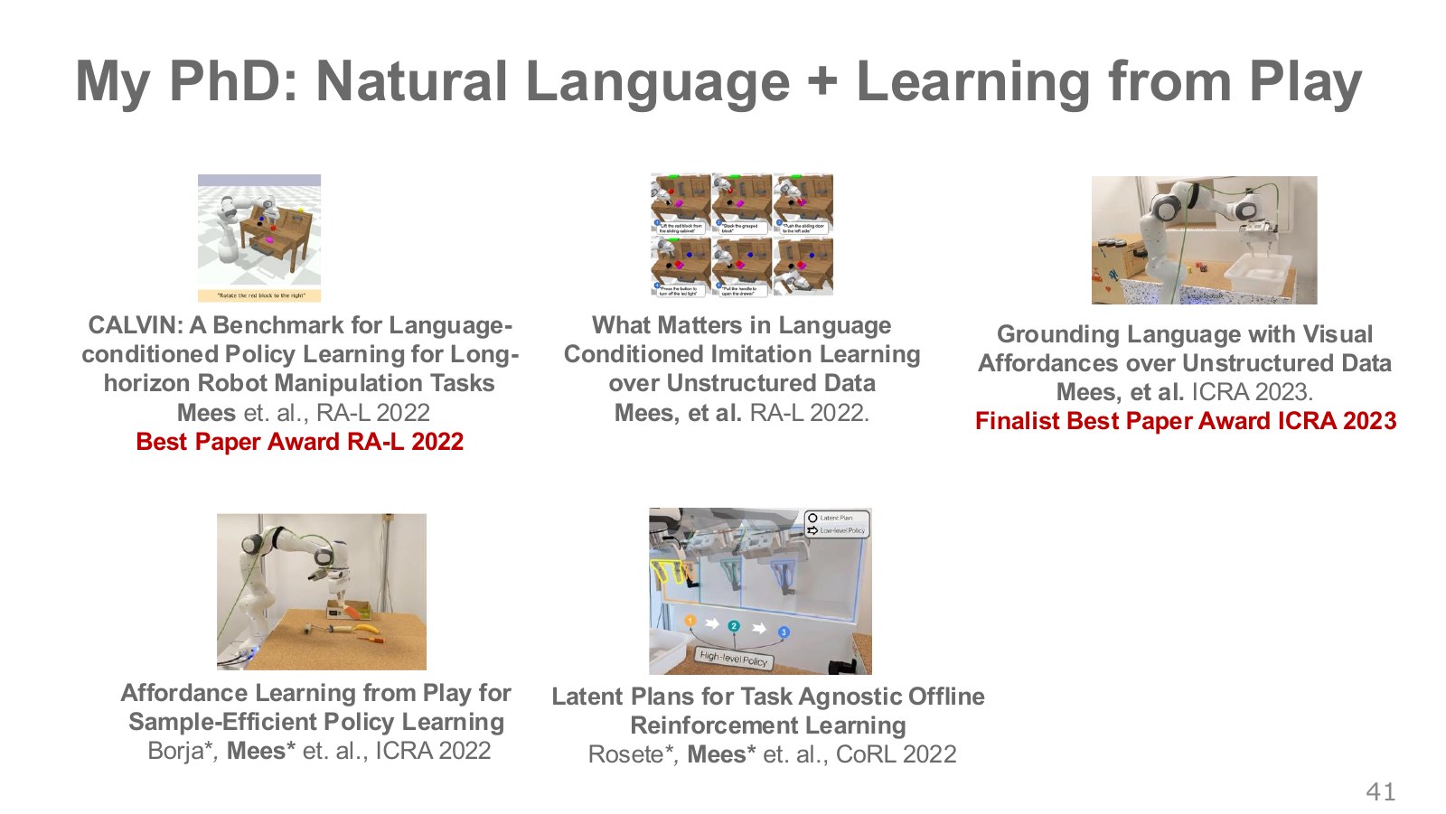
The studies above are not simply new policy names performing the same role. Distinguishing what each evaluates and learns makes them easier to connect to this chapter.
| Study | Question extending this chapter |
|---|---|
| CALVIN | How can we evaluate sequences of language-specified manipulation instructions? A benchmark supplying data and an evaluation environment. |
| What Matters in Language Conditioned Robotic Imitation Learning | How do representations, hierarchy and other design choices affect language-conditioned learning from play? |
| Grounding Language with Visual Affordances | How do we connect a sentence’s referent with the object region available for interaction? |
| Affordance Learning from Play | Can learning which regions people touch in play records help subsequent policy learning? |
| Latent Plans for Task-Agnostic Offline RL | How can short latent skills learned through imitation be composed for longer goals? |
An affordance is an opportunity for action or interaction arising from the relationship between an object and an agent: a handle affords pulling, for example, and a button pressing. Identifying what an object is in pixels differs from estimating where and how to interact with it.
A benchmark specifies comparison tasks, data and evaluation rules; a learning algorithm obtains a policy from given data. Before mixing results from different environments, align success criteria, observations, actions and data conditions. Original lecture, 49:25–49:37.
#P043 · Choosing tools to match the cause of behavior-cloning failure
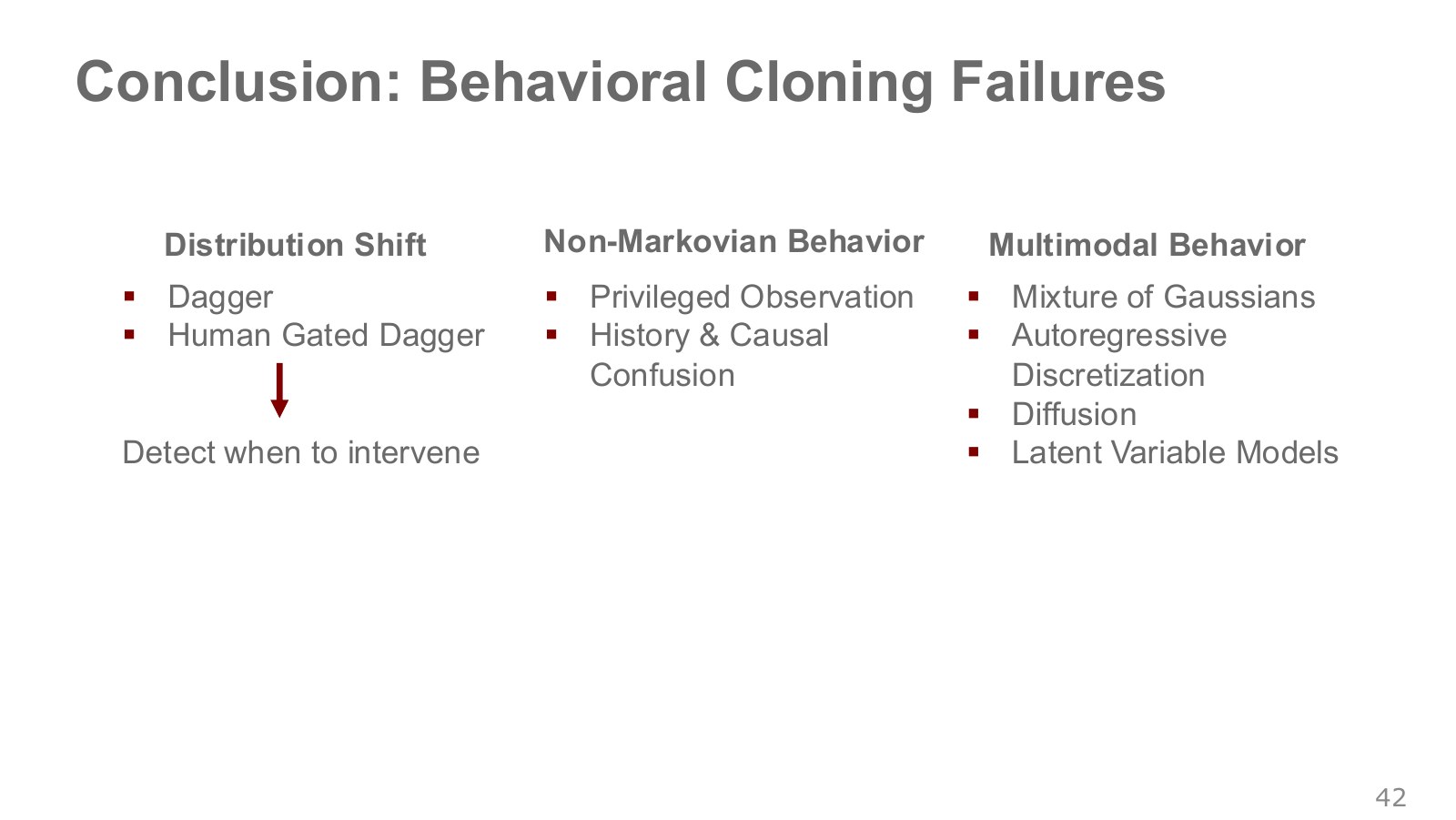
The final figure separates three causes. Before choosing the newest model, examine which best describes the current failure.
| Observed problem | What to check first | Relevant approaches |
|---|---|---|
| A small deviation leads to progressively worse mistakes. | Are good targets available for states visited during execution? | Recovery data, valid augmentation, DAgger and human intervention |
| The same photograph does not explain demonstrated actions. | Does the demonstrator have additional viewpoints, memory or goal information? | Align information and consider history models; also check reliance on easy spurious cues. |
| The policy selects the average between two valid actions. | Does the action distribution contain separated alternatives? | Mixtures, autoregressive discretization, diffusion or latent-variable models |
Several causes can coexist. A generative model representing multiple action modes can still lack the goal information needed to select one. DAgger can broaden input coverage while a model that collapses all actions to one average retains a representation problem.
This chapter’s criteria are good behavioral data, information actually available during execution, and a representation capable of expressing alternative actions. Separating them helps diagnose why a robot fails despite a small training loss. Original lecture, 49:39–50:27.
#Checking data coverage and equations with a small executable example
I published an executable NumPy one-dimensional synthetic environment. It isolates the process of labeling policy-visited states, without reproducing a real robot or the ETH assignment environment.
State is lateral deviation from target zero. The next state adds the policy action and a small disturbance to the current deviation. The policy is a linear function with output clipped to −1 through +1. Expert targets use under the same limits.
The initial dataset contains only twenty center-state/straight-action pairs . It cannot determine which slope should apply outside the center. The minimum-norm least-squares solution is . I then repeated policy execution, expert labeling of visited states and refitting three times. In this example, the first additional round identified slope −0.8.
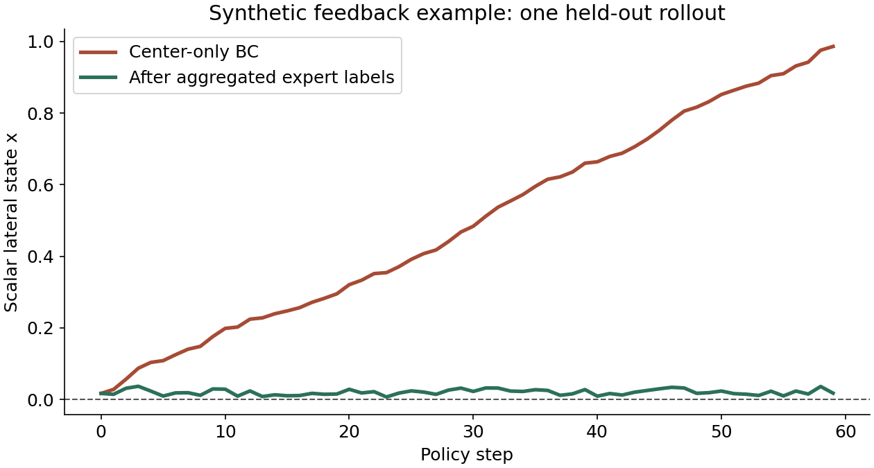
| Policy learned in this synthetic environment | Learned slope | Mean state RMS over 20 held-out evaluations |
|---|---|---|
| Center-only data | 0 | 0.415916 |
| Aggregated expert labels on visited states | −0.8 | 0.035215 |
RMS takes the square root of the mean squared state deviation within each run. The table averages that quantity over 20 evaluations. Each run has 60 steps, and both policies use the same seeds 1000–1019. State units are illustrative, not robot-arm position errors or success rates.
This difference arises from deliberately narrow center-only data and an expert with a linear target rule. It neither predicts the same improvement ratio for DAgger in every environment nor measures general neural-network BC performance. Its purpose is to make visible the loop of adding inputs generated by the learned policy back into training.
The same executable includes 15 checks covering MSE-optimal mean actions, mixture-density normalization, autoregressive probability sums, a compounding-error bound and the ELBO–posterior-KL identity. See the execution file, settings, result JSON and CSVs together.
#Continue with real robot-arm learning
The official ETH HW3 connects demonstration collection, behavior cloning, intervention data and goal-conditioned learning in SO-101 simulation.
| Official exercise | Concept to connect |
|---|---|
| Exercise 1, MSE policy | Collect teleoperation records, derive action labels from state differences and train a policy. Inspect observation/action coordinates and scaling. |
| Exercise 2, DAgger | Observe failures after changing obstacle distributions, add corrective human-takeover records and retrain. |
| Exercise 3, multiple cubes | Condition on target-cube color and destination-bin position. Check that goal information actually enters the observation. |
Because corrective collection uses online human intervention, distinguish it from basic DAgger’s labeling of every visited state. Success criteria should also distinguish a gripper reaching its target from an object actually being placed inside the bin.
I read the official assignment and code as references; these notes do not report training those policies or operating a real robot. The synthetic environment and numerical checks above are what I ran. For larger demonstration-learning examples, continue with Diffusion Policy’s public code and notebooks.
Chapter 04 turns from treating demonstrated actions as targets to the first reinforcement-learning algorithms that improve policies through rewards from acting in an environment.
#Sources and further reading
- Oier Mees — ETH Robot Learning, Lecture 3 · Video · PDF · Image copies
- Sergey Levine — Berkeley CS285, Supervised Learning of Behaviors · Compounding-error video · Practical BC video · Goal-conditioned learning video
- Hung-yi Lee — NTU imitation learning
- Ross·Gordon·Bagnell — DAgger, AISTATS2011
- Bojarski et al. — NVIDIA End to End Learning for Self-Driving Cars
- Giusti et al. — Forest Trails
- Mees·Burgard — Composing Pick-and-Place Tasks By Grounding Language
- de Haan·Jayaraman·Levine — Causal Confusion
- Lynch et al. — Learning Latent Plans from Play · Project
- Berkeley CS285 — Variational Inference and Generative Models · Kingma·Welling — Auto-Encoding Variational Bayes
- Chi et al. — Diffusion Policy · Official ETH HW3
P numbers follow the slide-image copies. Administrative, transition-only, closing and references-only slides are omitted. Copyright belongs to Oier Mees and the rights holders of incorporated material. Supplementary NVIDIA and Play-LMP diagrams belong to their original creators. The directly computed graphs and synthetic example are separate explanatory materials.