Reinforcement Learning 09 — Generalist Robot Policies

Even the same instruction to grasp a cup comes with different views and commands across robots. One has a wrist camera; another only a workbench camera. Some recordings encode an open gripper as 1, others as 0. Previous chapter: World Models

The explanation follows the official course schedule and automatic video captions. Figures follow the public image copies’ order. The official PDF is password-protected, so correspondence between its internal pages and the image copies could not be verified. Official ETH schedule · Official PDF · Slide-image copies

#Starting with one task on one robot

#P001 · Generalist robot policies

This is the recording for week nine on the course website. The copied cover says Lecture 10; this article follows the official schedule’s week numbering.

Original lecture, 0:00

#P002 · Strengths of specialist policies

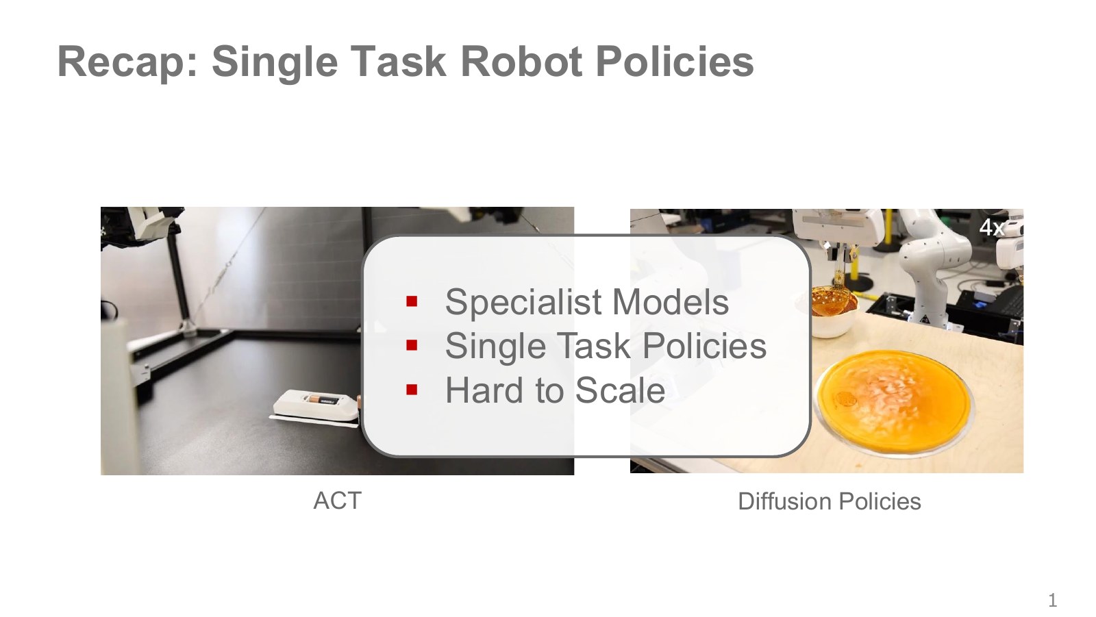
For inserting a cable with one arm type, ACT or Diffusion Policy can learn precise task-specific movements. Repeating training for each new camera or arm increases costs as tasks and hardware multiply.

Original lecture, 0:36

#P003 · Three axes of generality

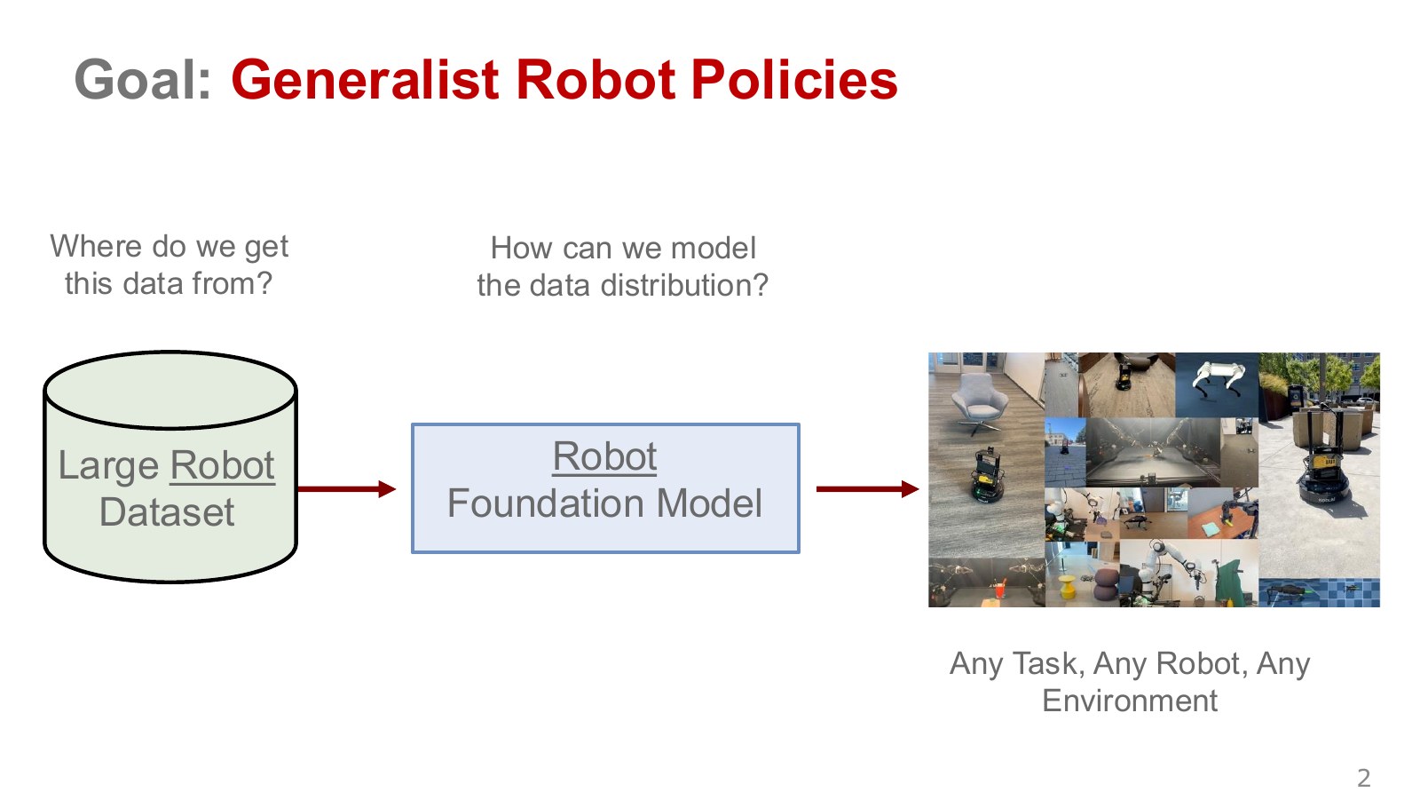
A policy maps current scenes and instructions to actions. Success on new objects, in new environments, and on new robots are different tests. Grasping an unfamiliar cup with an existing arm requires different adaptation from connecting a new arm.

Original lecture, 1:46

#P004 · The goal of an installable robot brain

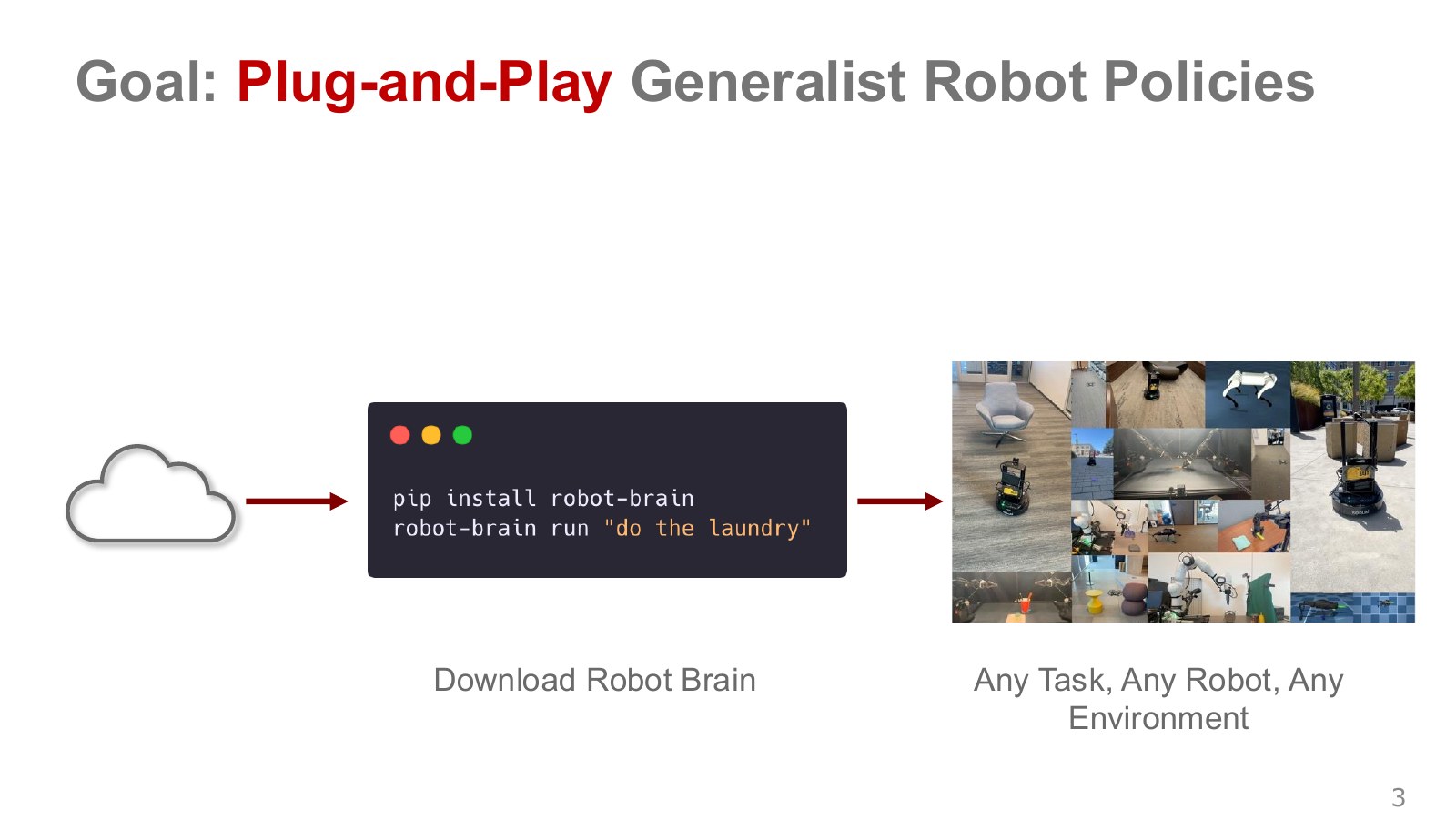
The terminal illustration depicts the research goal of controlling multiple devices through a simple installation. Actual integration still requires matching camera order, coordinate frames, control rates, command units, and hardware motion limits.

Original lecture, 2:30

#P005 · An idea borrowed from language models

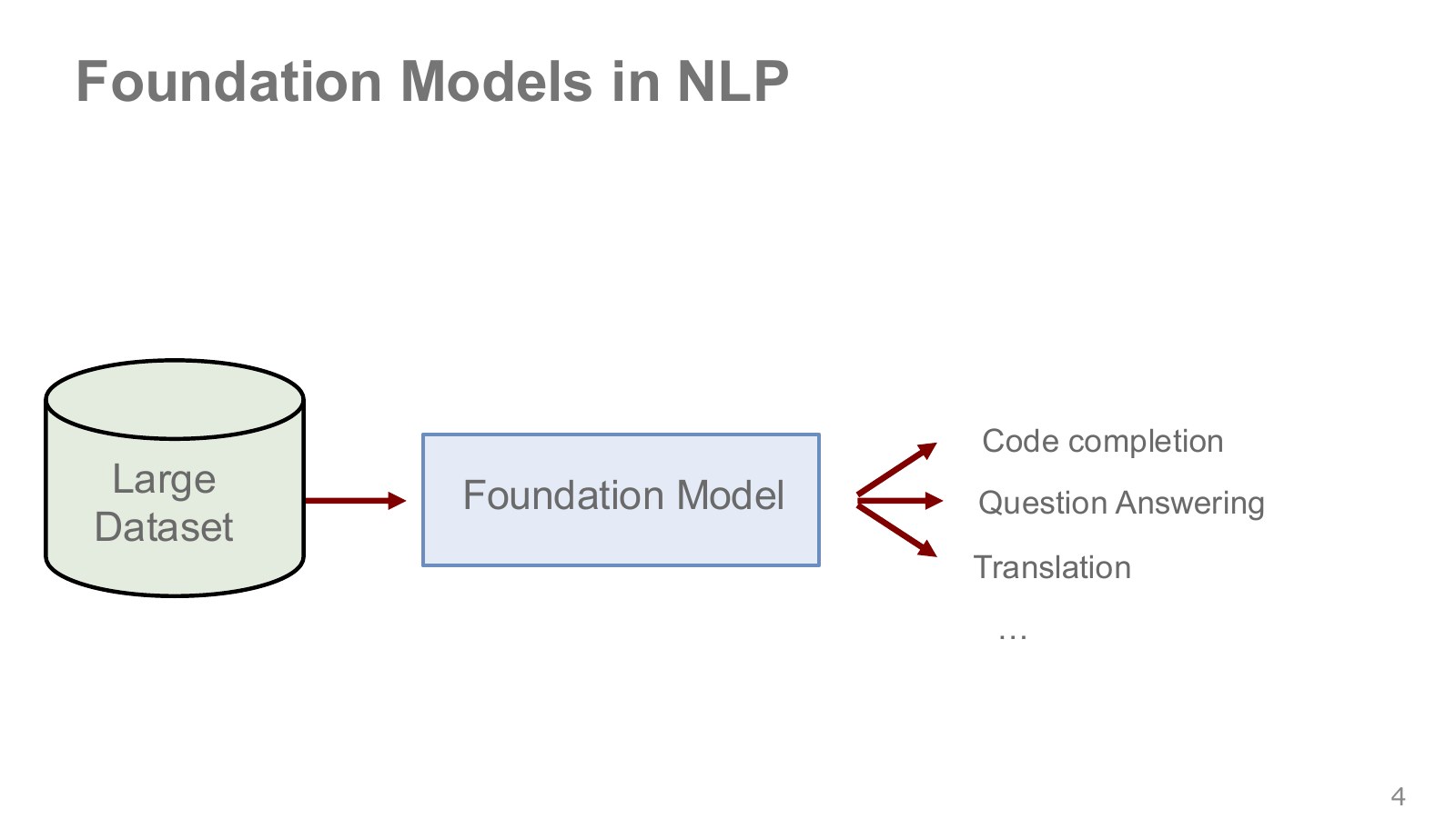
Representing tasks with different inputs and outputs, such as code completion and translation, as token sequences enables shared representations within one model. Robot images, instructions, and movements can likewise become learning units, but final outputs must remain executable by physical hardware.

Original lecture, 3:12

#P006 · Comparing generalist and specialist models

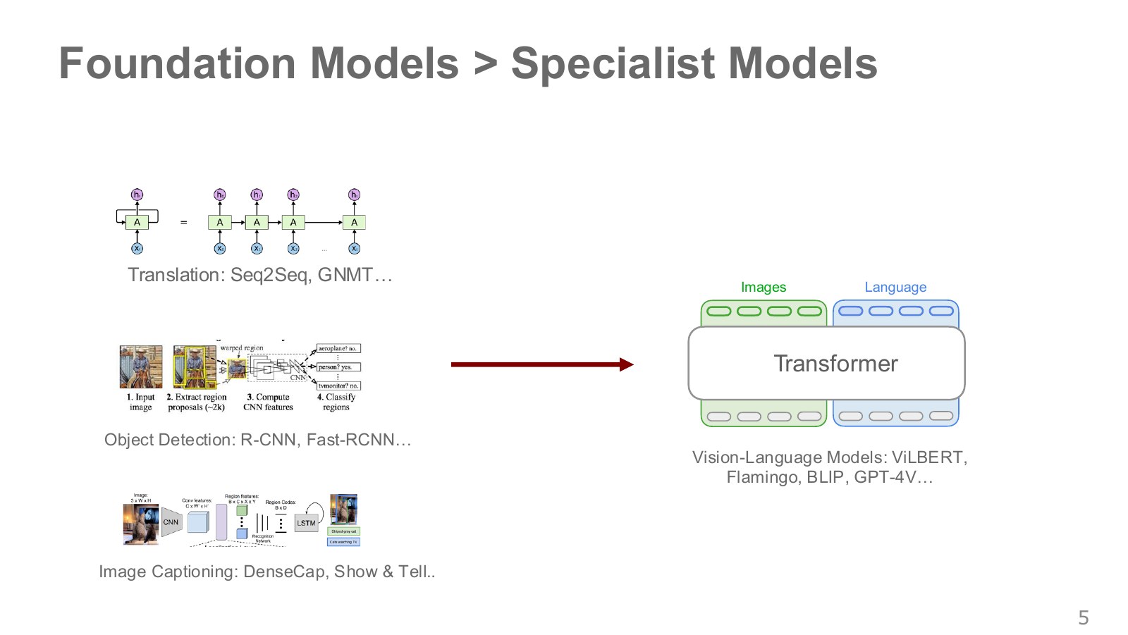
Translation and object-detection illustrations show a shift from dedicated models to shared models. Robot generalists must be compared directly with specialists on success and execution speed for the same tasks to establish the benefit.

Original lecture, 3:53

#P007 · Data, models, and evaluation

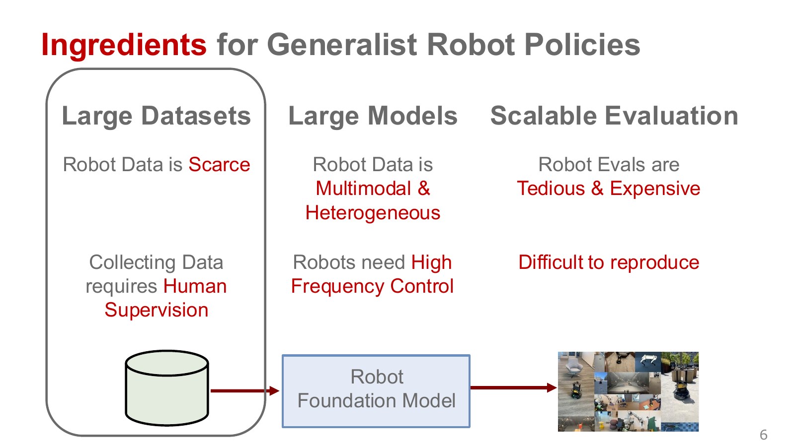
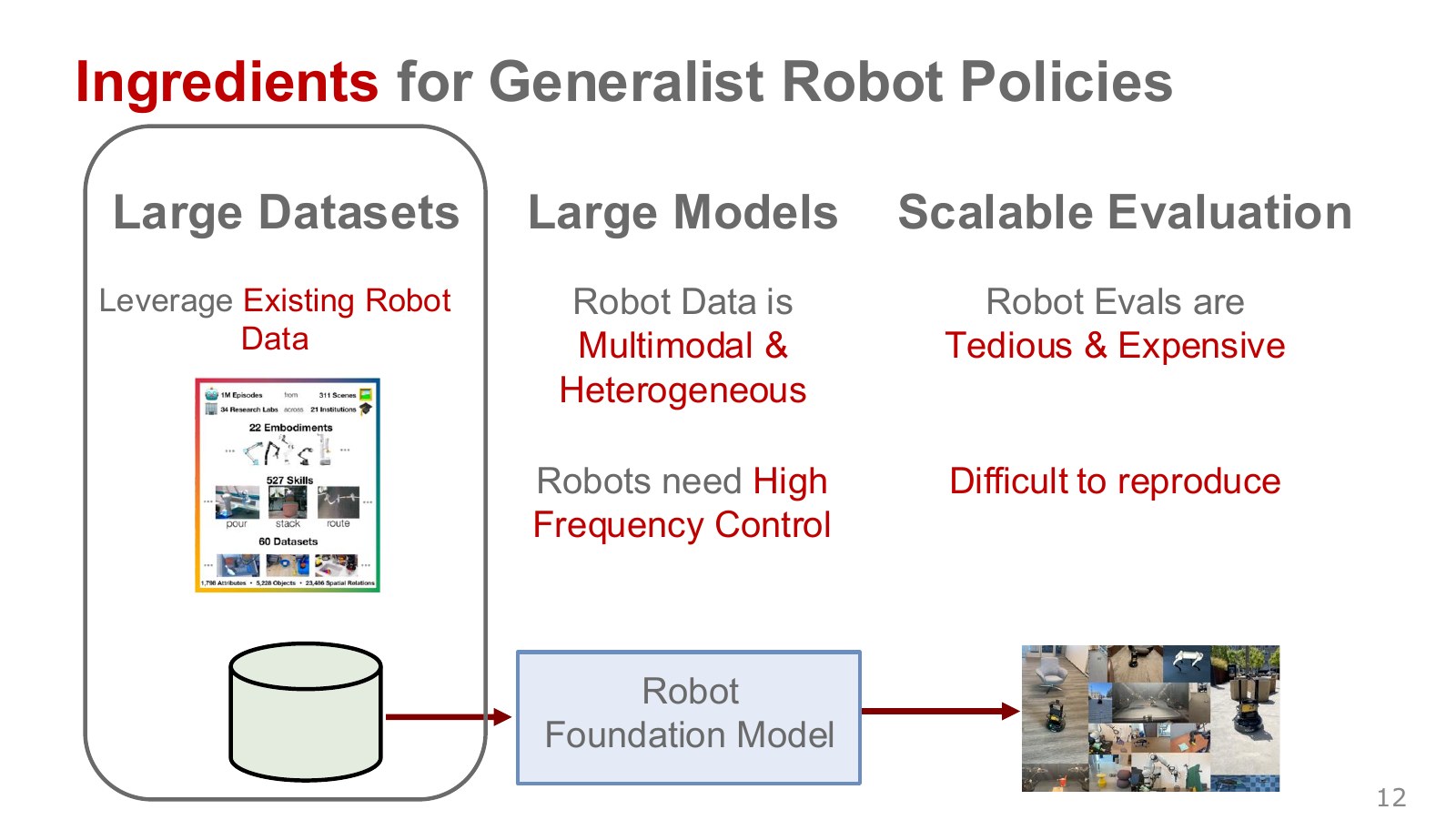
We need ways to collect experience across equipment, architectures accommodating input/output differences, and evaluations repeatedly measuring performance across those differences.

Original lecture, 4:22

#Bringing heterogeneous demonstrations together

Execution and evaluation constrain progress alongside data scarcity. Updating targets at 50 Hz leaves 20 ms per cycle. If a large model takes longer, a system needs separate fast low-level control and slower high-level decisions, action chunks, or asynchronous execution. Adding robots, objects, locations, and instructions also multiplies evaluation combinations. Generalist-policy scaling changes not only collection effort but also the cost of repeatedly establishing where the model works.

#P008 · The cost of collecting demonstrations

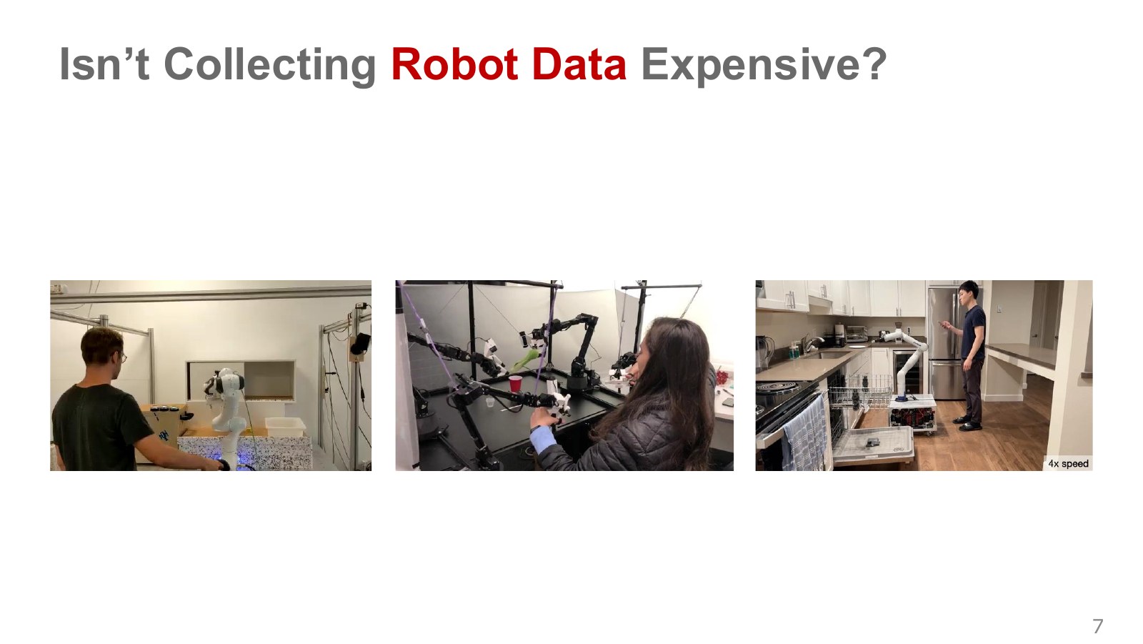
Recording one teleoperated cup placement requires arranging initial positions, resetting after failures, and synchronizing sensor and motion records. These physical repetitions create costs unlike collecting web documents.

Original lecture, 5:02

#P009 · Putting existing data into a common format

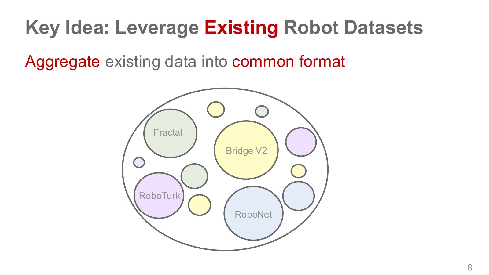
Despite different laboratory recording methods, an episode can expose observations and actions in time order. A common storage format aligns data access, while coordinate and semantic transformations remain separate.

As with the lecture’s tactile-laboratory example, small datasets originally collected for individual papers can be combined with other laboratories’ records. Mees recalls teleoperating a Franka during his PhD and describes the cost of recording all demonstrations afresh for each task as a motivation.

Original lecture, 8:21

#P010 · Open X-Embodiment

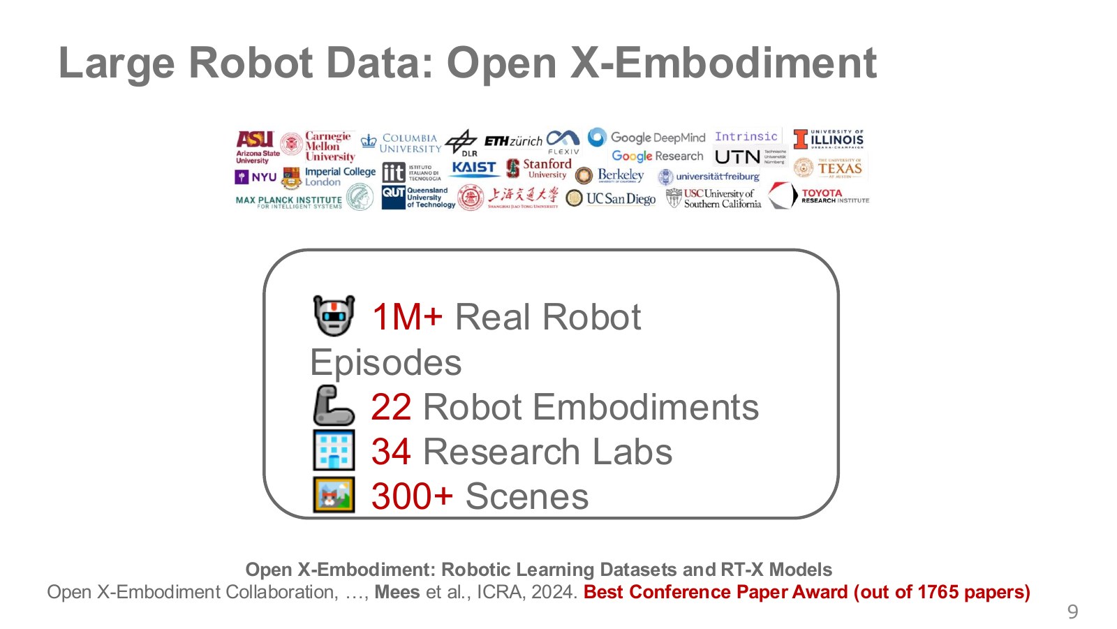
Manipulation records from multiple institutions support joint training. To understand what transfers, examine robot types, task overlap, and camera configurations alongside episode counts. Project

The Open X-Embodiment paper reports more than one million real episodes across 22 robot types. This describes the collected dataset as a whole. Octo’s approximately 800,000 episodes below are the subset used in that model’s pretraining. Open X-Embodiment paper

Original lecture, 9:20

#P011 · Checking transfer across hardware

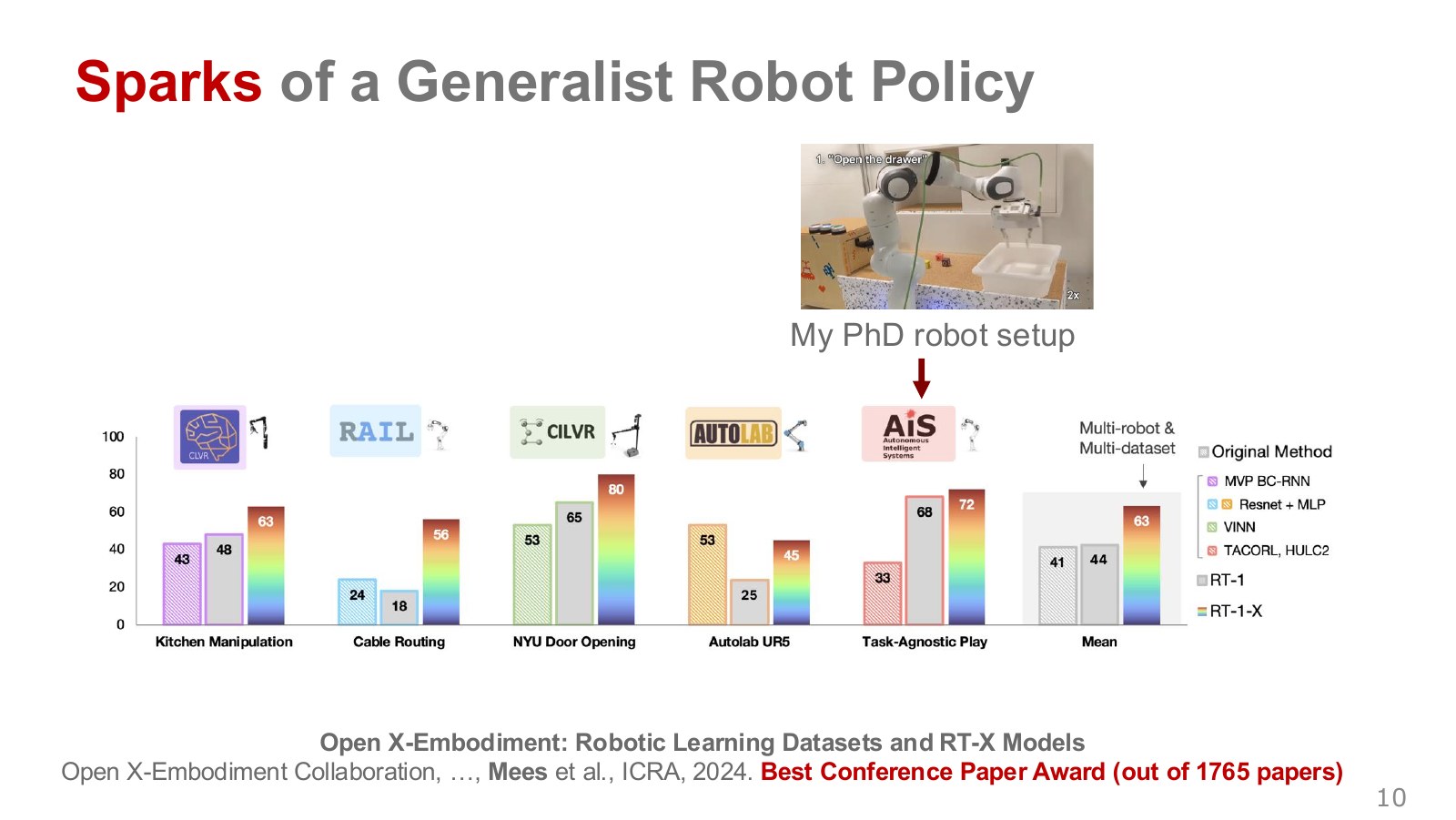
Distinguish training scenes from test scenes when viewing manipulation videos from different laboratories. Handling new objects on existing hardware and adapting to new hardware each require their own evidence.

Original lecture, 10:00

#P012 · From shared data to multiple policies

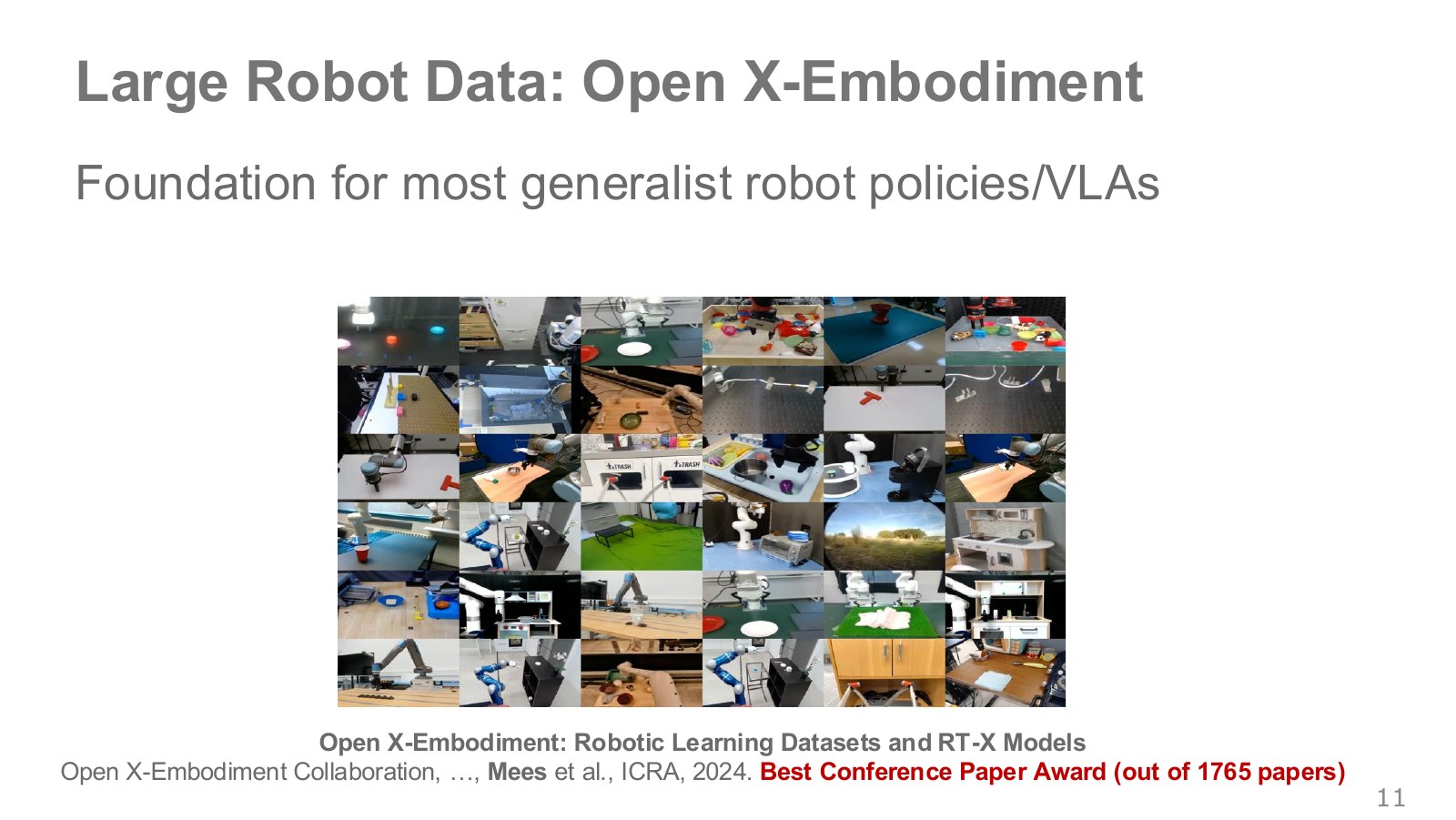
OXE enabled later policies to reuse parts of its data. Published total episode counts and episodes actually used by individual policies differ according to selection and filtering.

Original lecture, 11:02

#P013 · Models that read heterogeneous data

Jointly training arms with one camera and arms with wrist cameras requires accepting both input configurations while identifying missing observations.

Original lecture, 11:30

#P014 · Sensors and action spaces

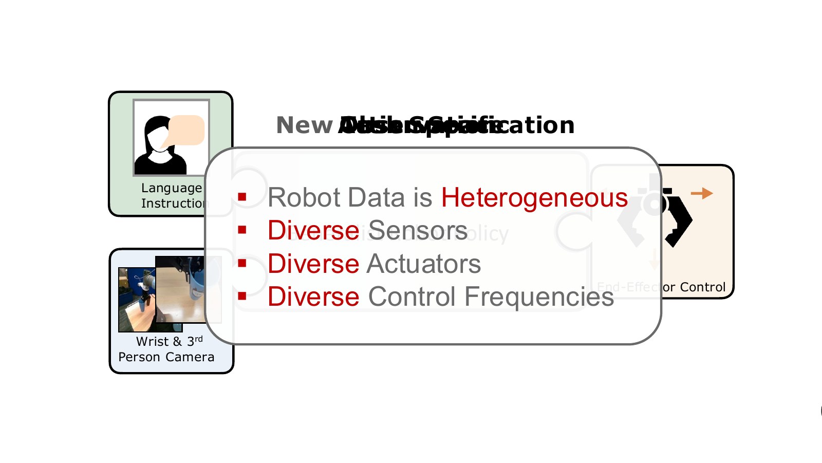
External and wrist cameras view the same cup from different positions. The same numerical output might mean fingertip displacement for one robot and joint velocity for another. Input and output differences require separate handling.

Original lecture, 11:46

#P015 · From instructions to movement

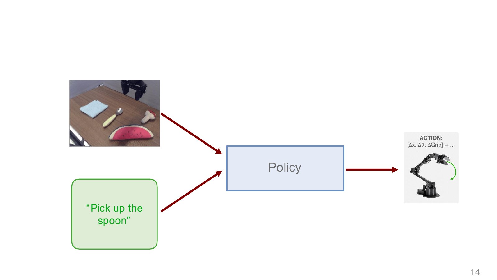
Given a photograph and an instruction to pick up a spoon, the policy identifies the object and decides where to move the hand.

Original lecture, 12:21

#P016 · From pictures to answers

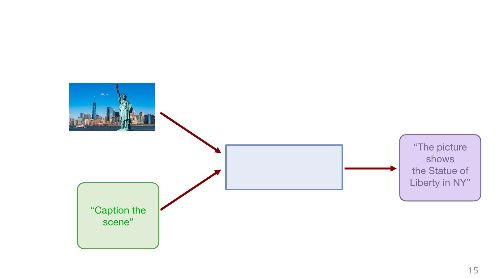
Asked to describe the Statue of Liberty image, a vision–language model connects images and sentences. This illustrates an input format similar to robot instructions.

Original lecture, 12:57

#P017 · Connecting VLMs to action policies

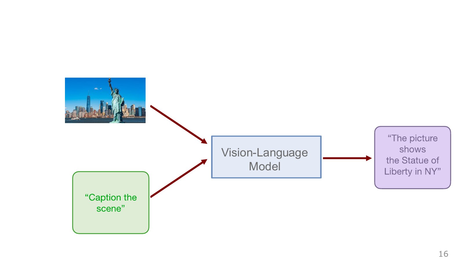
A VLM outputs descriptive text. Building an action policy trains its representations to predict control values such as fingertip motion and gripper opening.

Original lecture, 13:20

#P018 · Multiple token types in one model

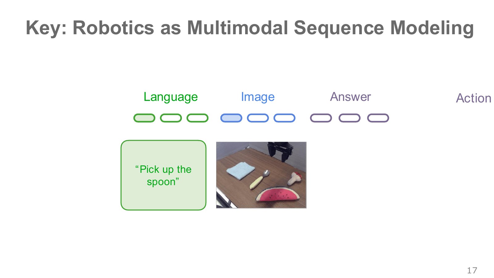
Image patches and instruction words become vectors that reference one another through a Transformer. Actions can be tokenized too, or produced by a separate continuous-output module.

Original lecture, 13:31

#How Octo turns goals and observations into actions

#P019 · Octo's training coverage

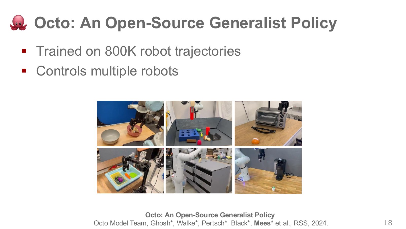
Octo is an open policy trained on about 800,000 episodes selected from OXE. It accepts language instructions or goal images, and is evaluated directly on represented hardware or fine-tuned with data from new hardware. Octo project

Original lecture, 14:30

#P020 · Task tokens and observation tokens

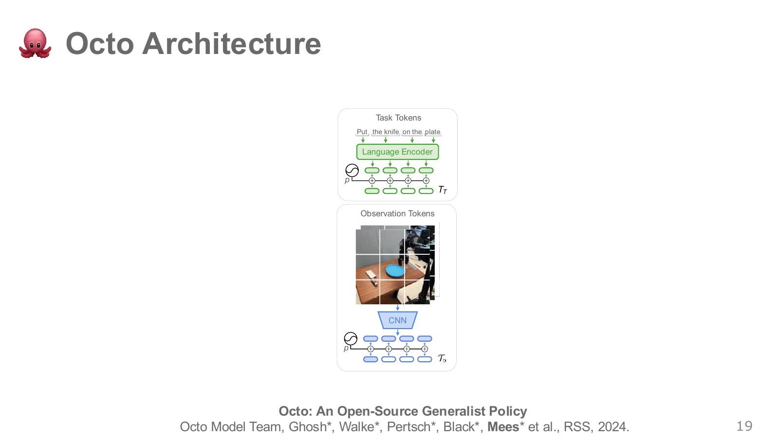
“Place the knife on the plate” specifies a goal; external and wrist images show current positions. Following the two diagram paths separates what to do from where things are now.

Pretrained T5 represents language, while a small convolutional encoder converts images into observation tokens. A Transformer reads both and gathers action-generation information into purple readout tokens. Their numerical values are passed to a diffusion head rather than directly to motors. Octo paper

Original lecture, 15:13

#P021 · Time direction and permitted references

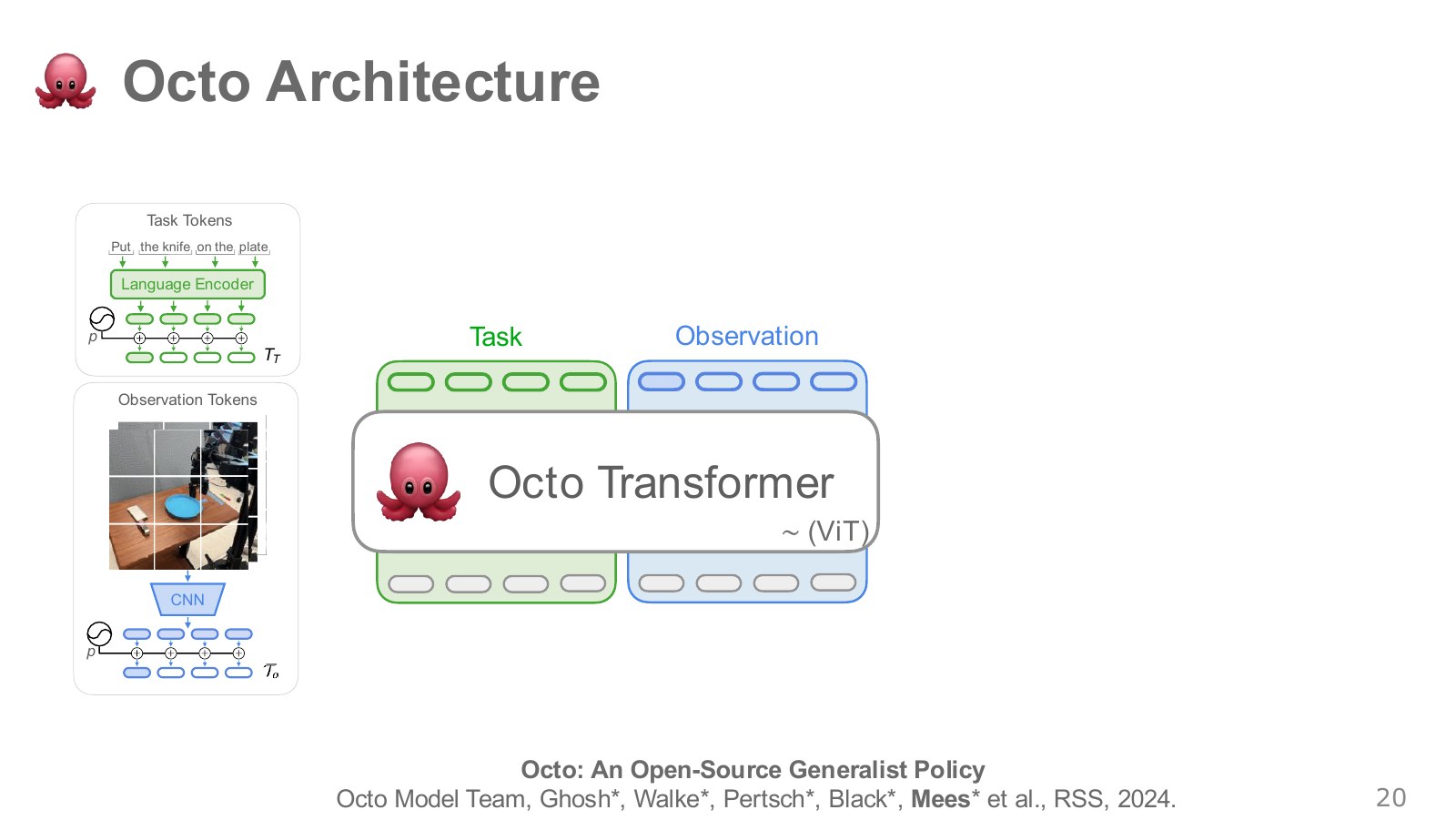
Octo uses block-causal attention. Representations generating current actions read past and current observations, preventing references to future camera frames unavailable during execution.

Original lecture, 16:10

The block-causal structure defines both temporal constraints and token roles. Cameras at the same time can reference one another, and current observations can read goals and earlier observations but not future ones. Readouts aggregate goals and observations for output heads. Reference directions also prevent observation or output-readout information from flowing backward into goal representations. Rather than summarizing every mask with the transcript’s sentence “task tokens cannot reference each other,” consult the paper’s token-type permission table. Octo paper

#P022 · Imitating demonstrations conditioned on a goal

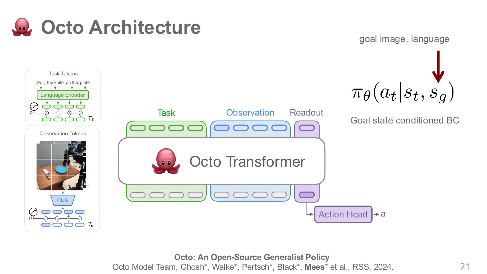
With a goal-state image, the difference between a completed knife-on-plate image and the current image informs action selection. Language goals likewise condition the policy.

Original lecture, 16:46

#P023 · Action chunks from a diffusion module

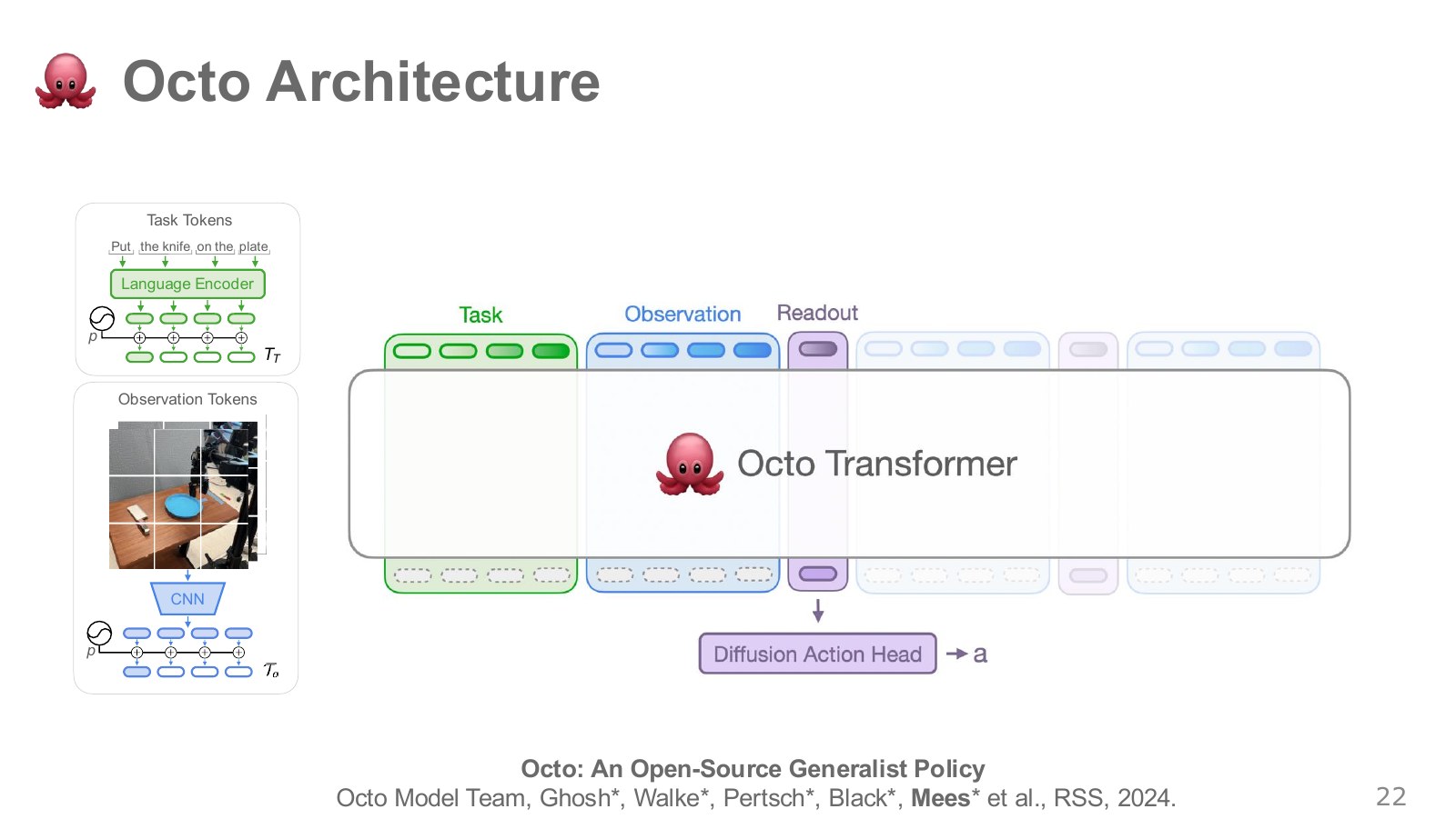
The action module receives information aggregated in readout tokens and generates multistep continuous controls from noise. A distribution helps represent approaching the same cup from the left or right.

Original lecture, 17:20

#P024 · Aligning the meaning of gripper values

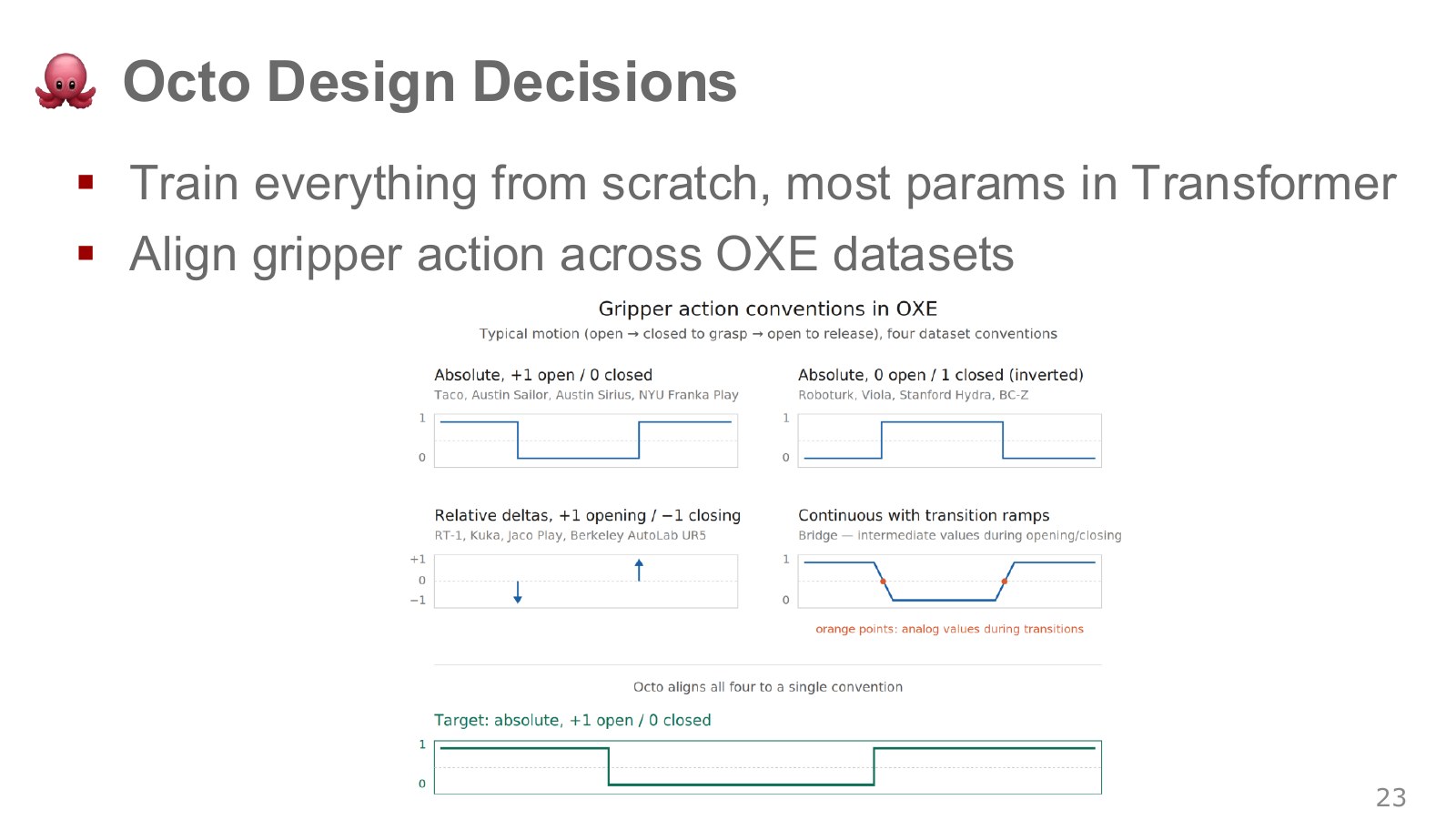
In one dataset, 1 means open; in another, closed. Other datasets store continuous values or change directions. Opposite binary absolute conventions can be aligned by inversion, while relative commands require examining opening/closing events and state.

Original lecture, 18:55

Octo’s common convention is open=1 and closed=0. But alignment goes beyond flipping numbers: datasets may record current aperture, a relative “open farther” command, or binary closure. Recovering absolute opening state from relative commands may require reconstructing earlier history. Aligning this dimension after initial grasp failures illustrates that even a large Transformer does not automatically reconcile opposite target meanings. It does not mean every dataset’s coordinate frames were fully standardized.

#P025 · Direct execution and fine-tuning

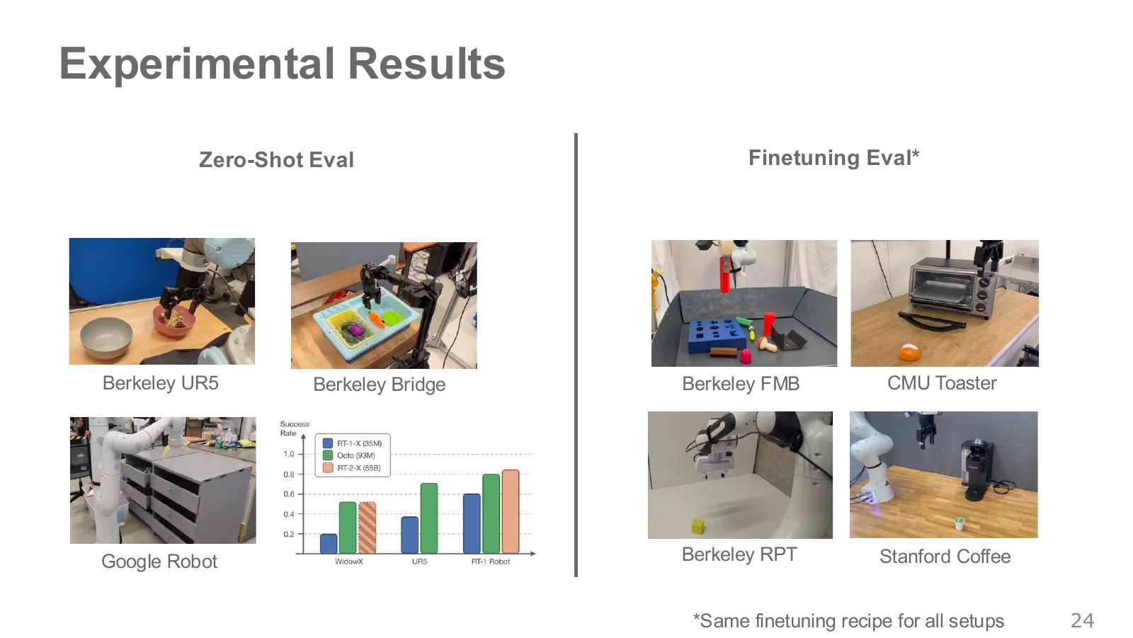
Zero-shot results use a model without additional training on new demonstrations for that evaluation. Fine-tuned results for coffee making or precision insertion follow training on those tasks’ data. The two figure groups therefore have different starting conditions.

Original lecture, 20:05

#P026 · Successes and failures behind the average

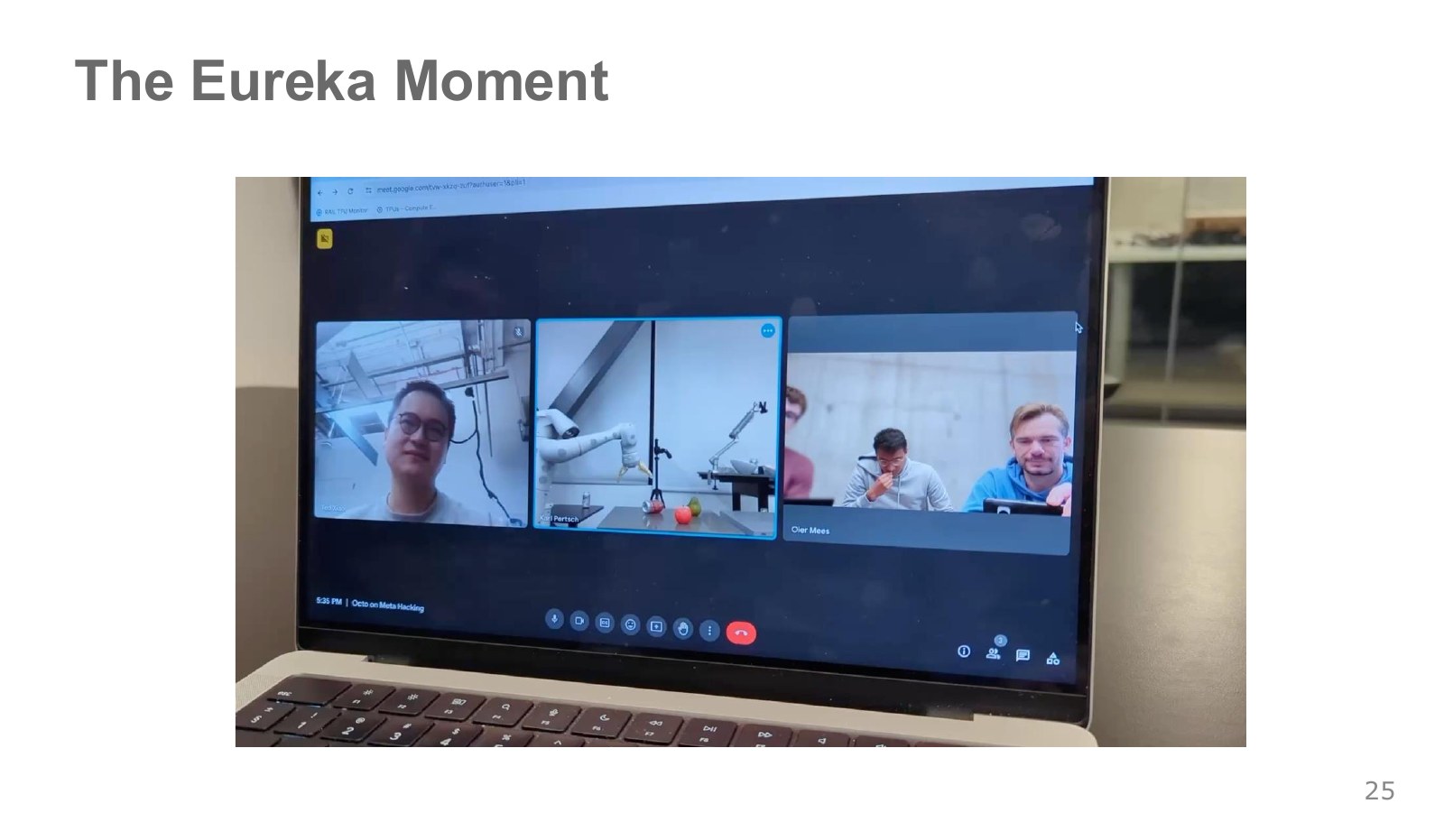
Videos revealing where a gripper closes and when an object slips can expose errors hidden by aggregate success rates. More hardware requires repeated trials and failure records by condition.

For the first Google-robot grasp shown, the policy ran on a remote server and Quan Vuong assisted with local evaluation. Google robot records were included in training, but testing occurred in another building. One successful video demonstrates operation at an unfamiliar location; success rate requires separate repeated trials.

Original lecture, 21:20

Rather than applying a large ResNet separately to every image before fusion, Octo concentrated computation in small image tokenizers and a shared Transformer. It initially learned representations from robot data alone. The lecturer revisits this choice because it differs from later reuse of Internet-scale VLMs. The paper’s gains over RT-1-X and comparability with the much larger RT-2-X concern its particular hardware, tasks, and data. Fewer parameters do not establish superiority for every semantic-understanding or new-hardware adaptation problem. Octo research team

#P027 · New cameras and command formats

Adding a wrist camera or force sensor changes input format. Outputting end-effector target poses instead of seven joint velocities changes output format too.

Original lecture, 22:20

#P028 · Change inputs and outputs while reusing representations

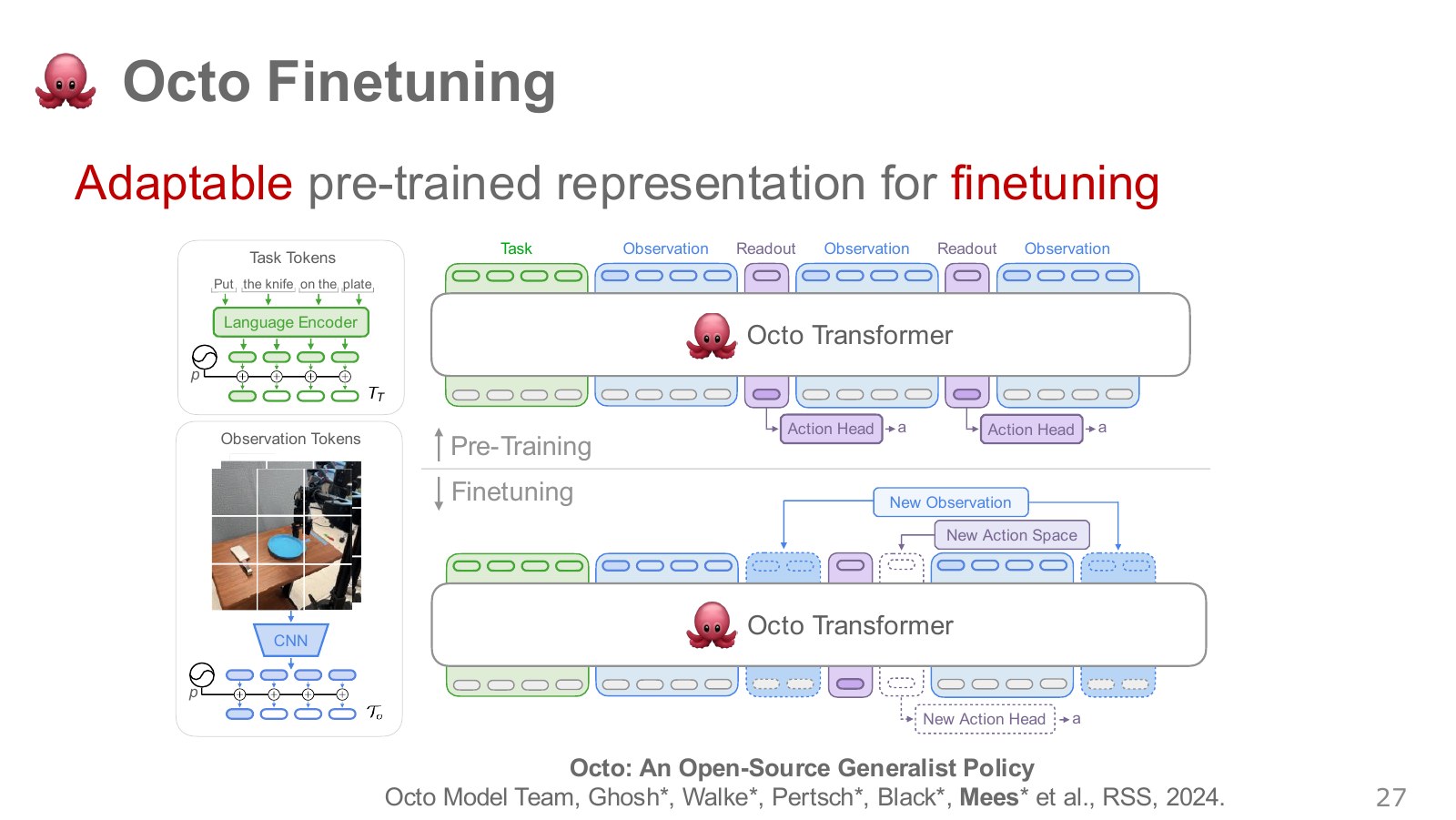
The upper Octo diagram shows pretraining and the lower fine-tuning. New sensor-tokenization modules and output heads are connected, using learned scene representations as initialization.

Original lecture, 23:14

#P029 · Adapting to new tasks with few demonstrations

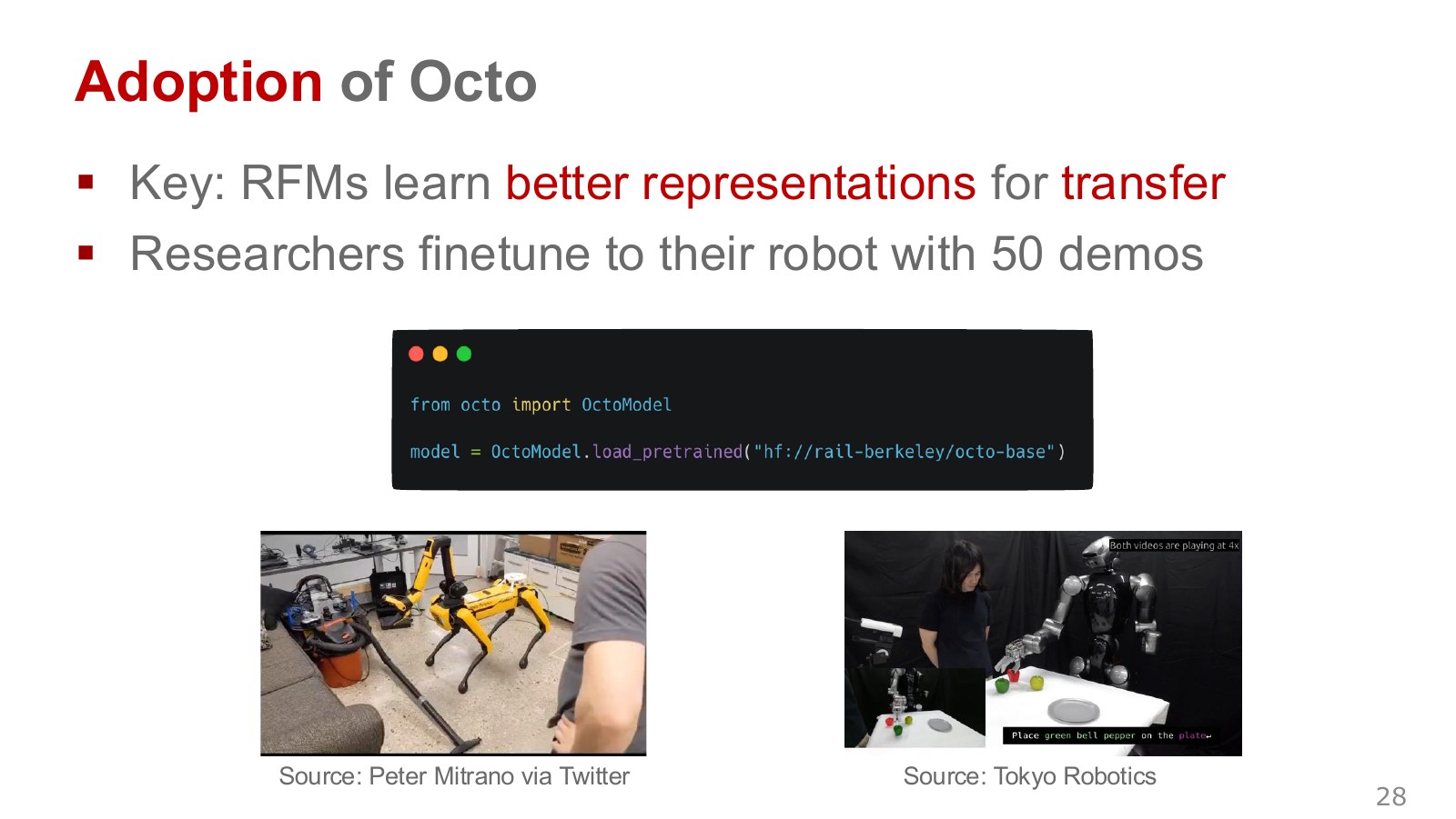
These demonstrations illustrate researchers starting from the released model. Approximately fifty refers to the scale of the cited application. Required demonstrations depend on task precision and relevance of pretraining data.

Original lecture, 24:34

#What can be shared across different embodiments?

A new force–torque sensor requires an input module converting its readings into tokens. Joint-target output requires an appropriately formatted head. Octo places most parameters in the shared Transformer and fine-tunes these representations together with new interfaces. The lecture contrasts starting from an entire policy pretrained on robot actions with starting from a backbone pretrained only on visual representations. Spot and Japanese-company humanoid examples are downstream adaptations to particular equipment, not evidence of unchanged-checkpoint zero-shot control on those robots.

#P030 · Generality beyond a single arm

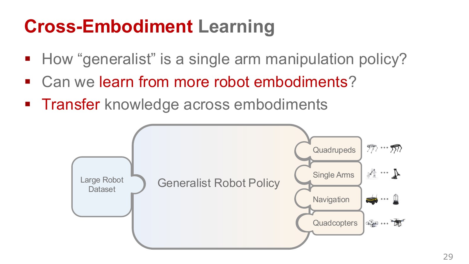
Wheeled navigation, quadruped locomotion, and drone flight differ greatly in observations and control. Testing such embodiments probes how much scene-reading representation can be shared.

Original lecture, 25:32

#P031 · Combining manipulation, navigation, walking, and flight

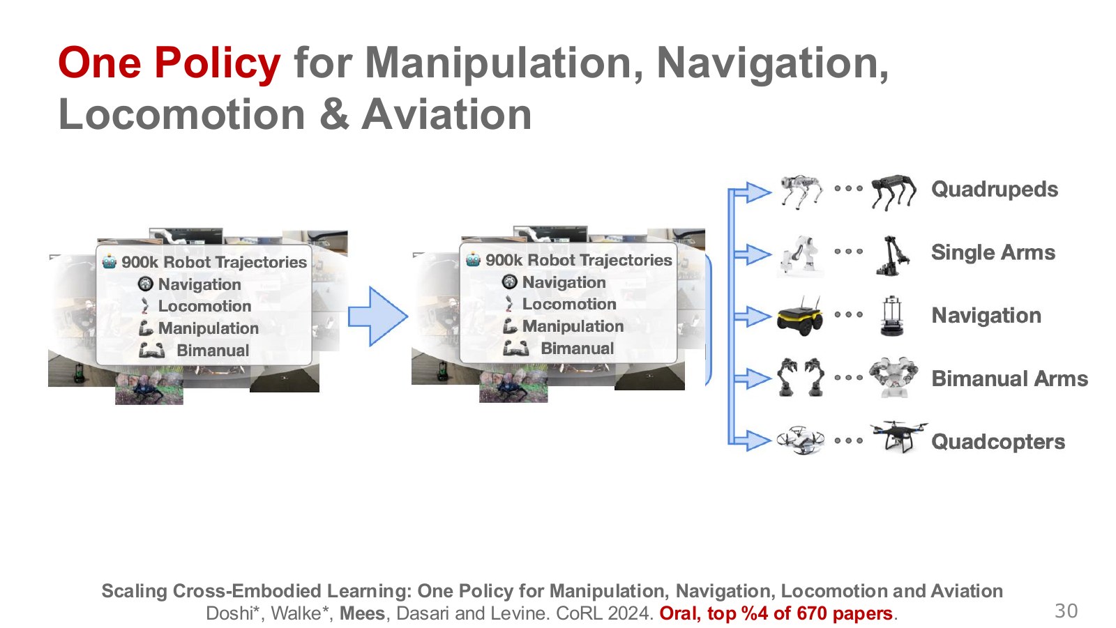
CrossFormer combines about 900,000 trajectories across embodiments in one policy architecture. Recognizing the same obstacle does not make an arm’s avoidance movement equivalent to a drone’s altitude change.

Original lecture, 26:34

#P032 · A shared backbone with embodiment-specific outputs

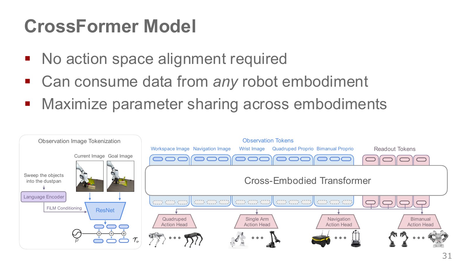
CrossFormer shares its Transformer backbone while assigning output heads by embodiment. A head converts shared representations into the equipment’s control vector. This permits joint backbone training without forcing drones and dual-arm robots to have identical action dimensions. CrossFormer project

The lecture’s examples control WidowX at 5 Hz and a dexterous dual-arm system at 50 Hz. Predicting one second therefore requires five versus fifty commands. Embodiment-specific heads can accommodate temporal resolution as well as control-vector dimension.

Original lecture, 27:05

#P033 · Multiple executions from one model

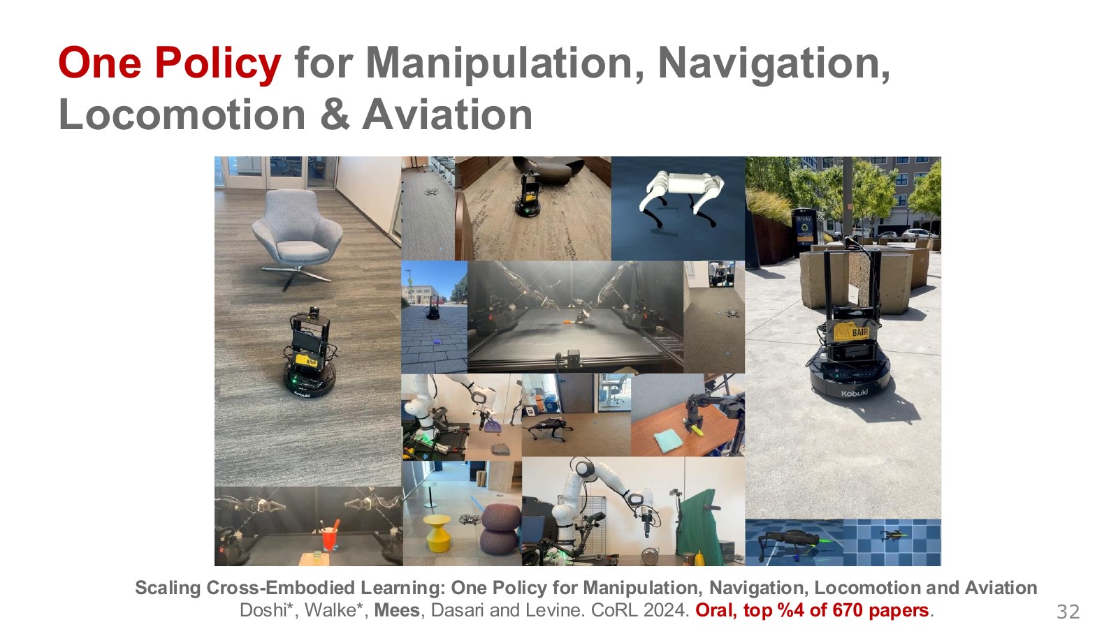
The videos use shared representations from the same checkpoint but different connected controllers. Distinguish execution on supported equipment from immediate control of unseen equipment.

Original lecture, 29:11

CrossFormer’s videos do not combine separately selected best checkpoints for each robot: they select embodiment-specific heads from one checkpoint. Shared parameters are used extensively, including shared encoders for matching camera types. Navigation experience may help visual obstacle representations, but this is not copying wheel speeds directly into quadruped joint torques. Separating shared representations from embodiment-specific action transformations clarifies the benefit of joint learning.

#P034 · Compare against specialists on each embodiment

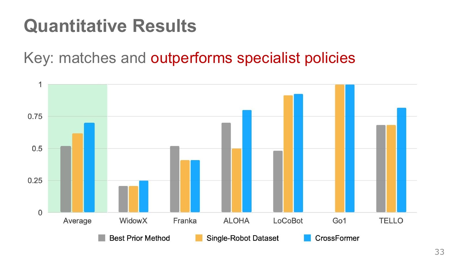
Embodiment-specific bars alongside averages matter. Large gains on some equipment can hide regressions elsewhere. Interpretation requires matched baselines, data, and trial counts.

Original lecture, 30:22

#P035 · Demonstration savings from pretraining

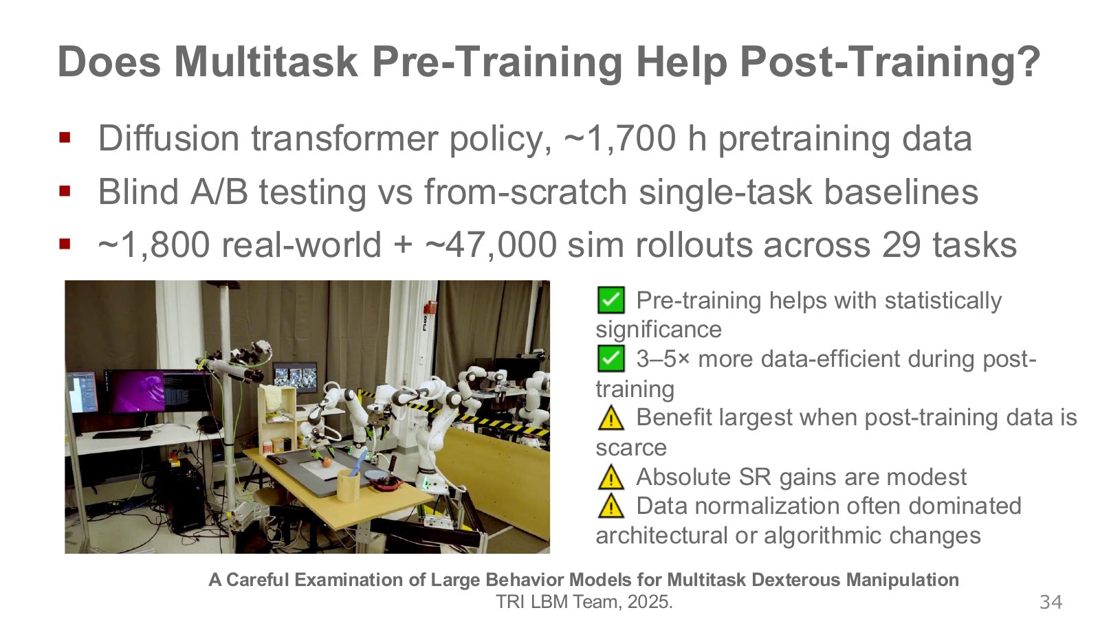
TRI compared pretrained policies with policies trained from scratch on 29 tasks. Some settings involving environmental variation required three to five times less new-task data. This does not mean success rates multiplied by that factor on every task. TRI source

In blind A/B evaluations, operators judged outcomes without knowing the policy identity. Pretraining helped particularly when post-training data were scarce, while normalization choices also affected outcomes. Data preprocessing must therefore be recorded among experimental conditions. TRI study

Original lecture, 30:57

#Transferring web-learned representations to robots

The TRI research introduced here studies diffusion-Transformer policies using about 1,700 hours of pretraining experience in real manipulation and simulation. Long dual-arm tasks such as peeling an apple offer more failure points than a short grasp. Blind evaluation and repeated trials separate pretraining effects from this variability. The observation that normalization can matter more than architectural changes underscores matching action units and preprocessing before comparing models. TRI study

#P036 · Using Internet-learned representations for control

Learning only from robot data may require demonstrations even to understand a new object name. Reusing web-learned image–word relationships can help locate objects, while robot records teach grasping motions.

Original lecture, 33:50

#P037 · LLaVA image tokens

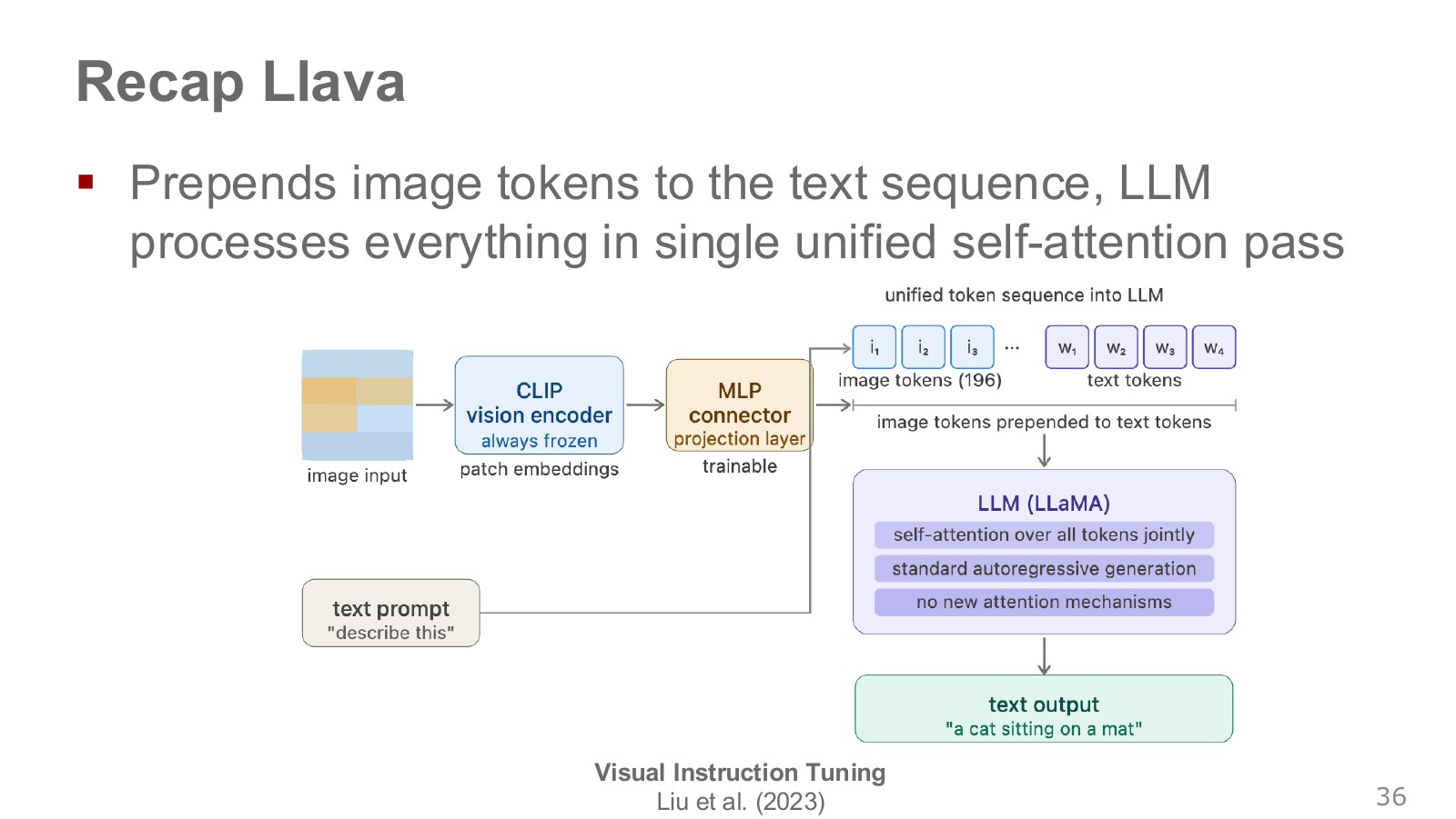
An image encoder converts a photograph into vectors, and a projection layer maps them into a dimension the language model can read. The model reads these alongside text in the same sequence. LLaVA project

Original lecture, 34:58

#P038 · Can actions also become tokens?

Connecting continuous motion to next-word prediction requires a rule mapping it to indices. Execution also requires a rule decoding those indices back into physical units.

Original lecture, 35:32

#P039 · From VLM to VLA

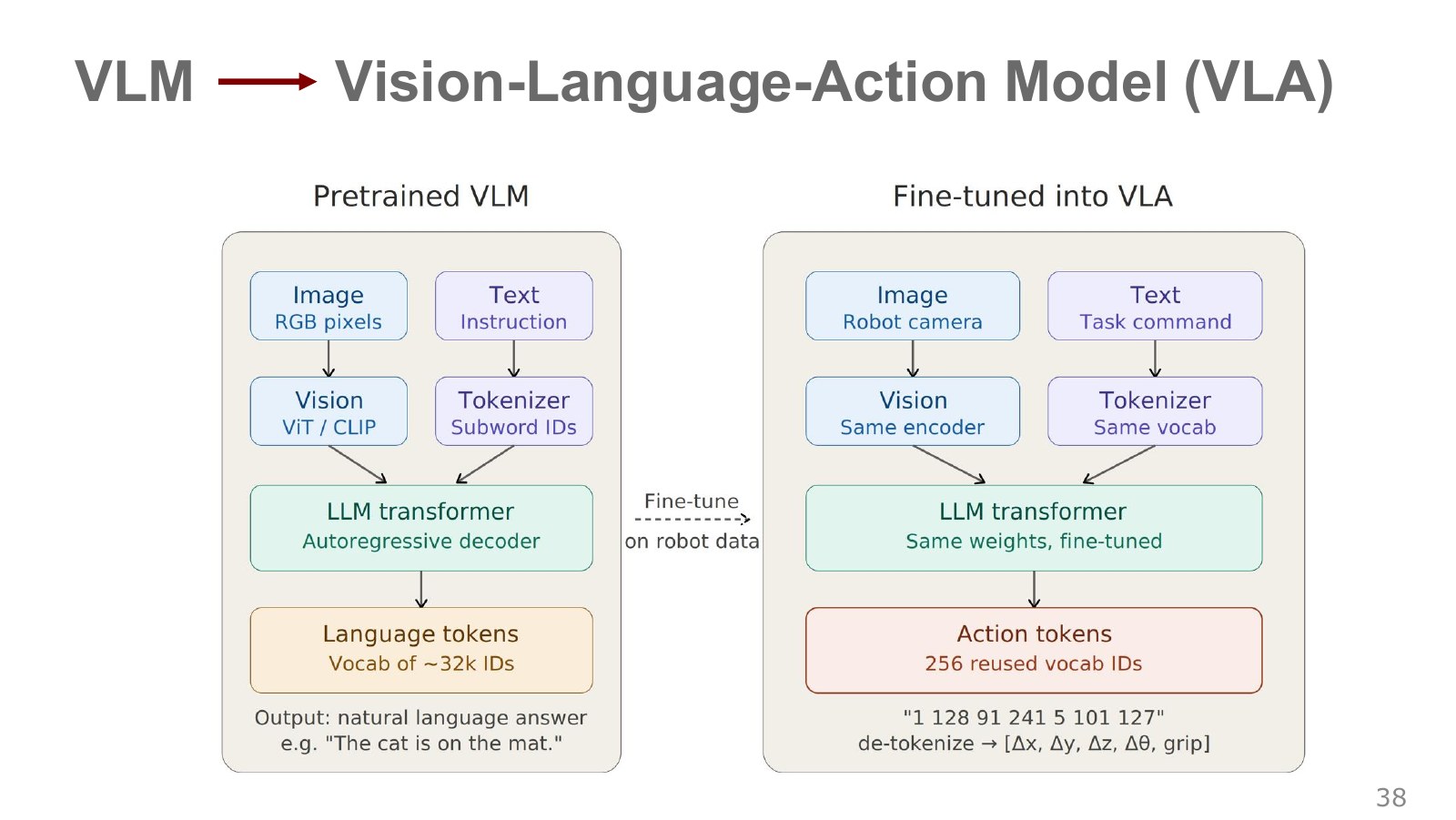
Adding action learning to a VLM produces a VLA predicting actions from instructions and images. Even with the same image input, descriptive text and physical controls require different training targets and data.

Original lecture, 36:04

#P040 · Clip by quantiles, then assign indices

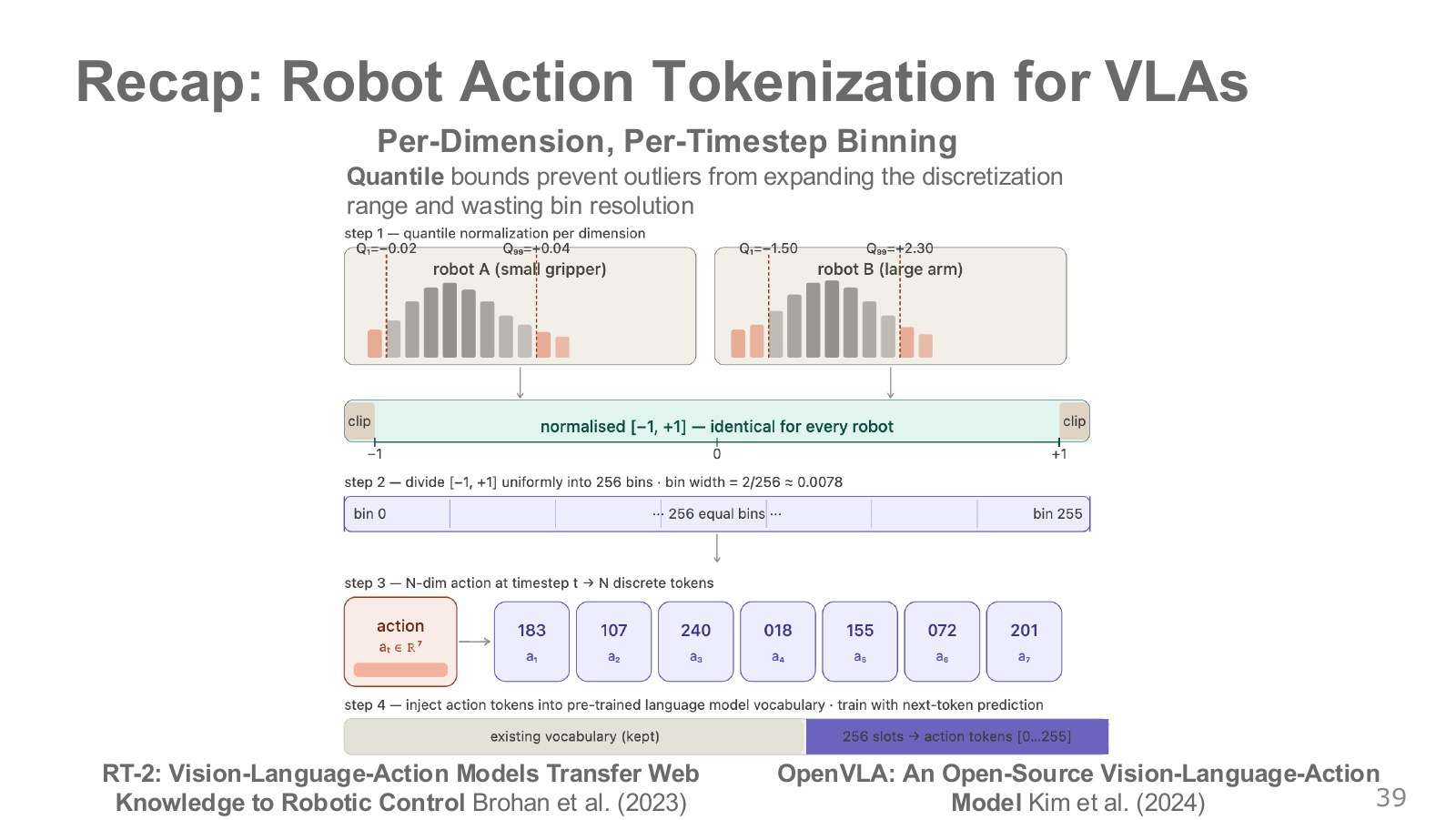
One extreme outlier can widen the full range and reduce resolution for common small movements. Set lower and upper references per action dimension, clip the range, then divide it into equal bins. The equation below simplifies the lecture’s 256-bin example. OpenVLA

Original lecture, 36:45

#P041 · Index accuracy versus physical error

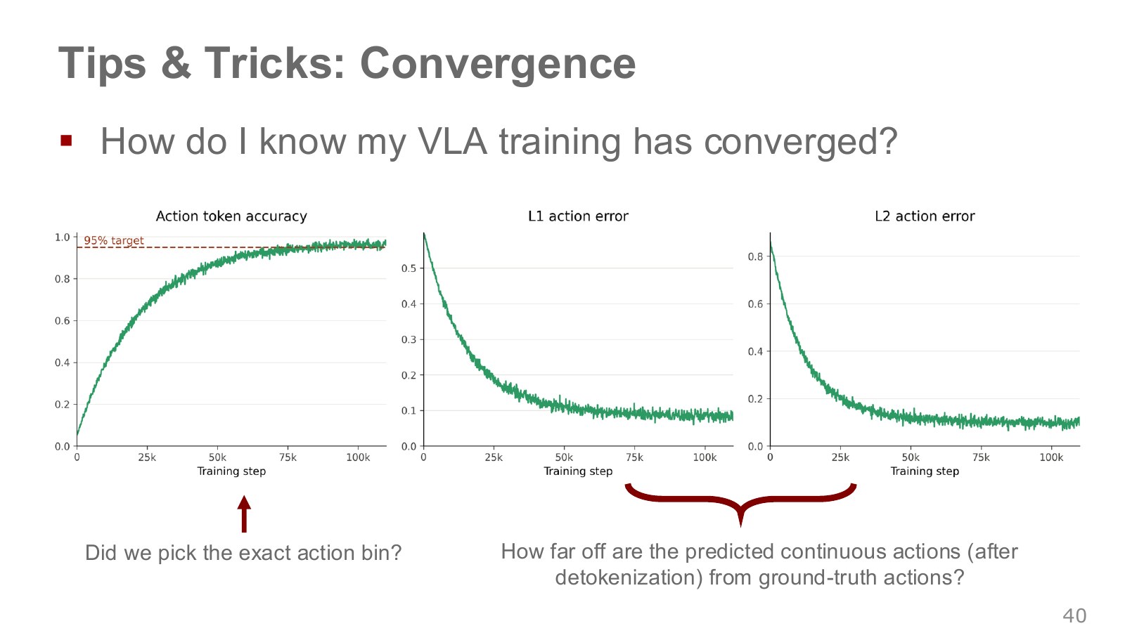
Choosing the bin next to the correct one still counts as a token error. Also evaluate the physical discrepancy after decoding. The equation below gives mean absolute error; when combining dimensions with different units, report per-dimension values or normalization conventions as well.

The lecturer’s approximately 95% is an empirical rule of thumb for monitoring autoregressive-model training. It is computed with teacher forcing, supplying correct preceding tokens, unlike rollout success under the model’s own predictions and actual sensors. This motivates examining decoded control error at the same checkpoint too.

Translate token accuracy into motion: a slightly-too-far leftward prediction counts as one token error. The same discrepancy has different consequences far from an object and immediately before contact with a thin glass cup. Examine token accuracy, per-dimension L1/L2 errors, and actual task success together. If rotations and translations were normalized to the same numerical range, their physical-axis errors should remain interpretable after decoding.

Teacher forcing may feed correct preceding action dimensions into later ones. Autonomous generation instead reuses preceding predictions. Thus a checkpoint’s training metrics and actual execution can differ. Treat the lecturer’s 95% guideline as a convergence clue while checking full object-transfer trajectories separately.

Original lecture, 37:40

#Training heterogeneous records together

#P042 · Padding and masks

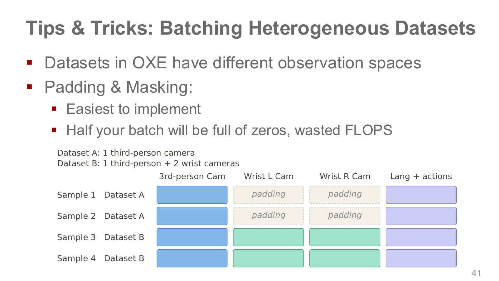
Empty positions can align a one-camera sample with a three-camera sample. A mask marks those positions as unobserved rather than measured. Standard dense computation still pays some cost for padding.

For example, padding samples with 100 and 300 camera tokens to length 300 gives 600 positions, of which 200 are empty. Attention masks prevent references but, depending on implementation, storage and computation remain. Padding simplifies formats; packing reduces empty positions but requires strict sample-boundary handling.

Original lecture, 39:00

#P043 · Reducing empty positions through packing

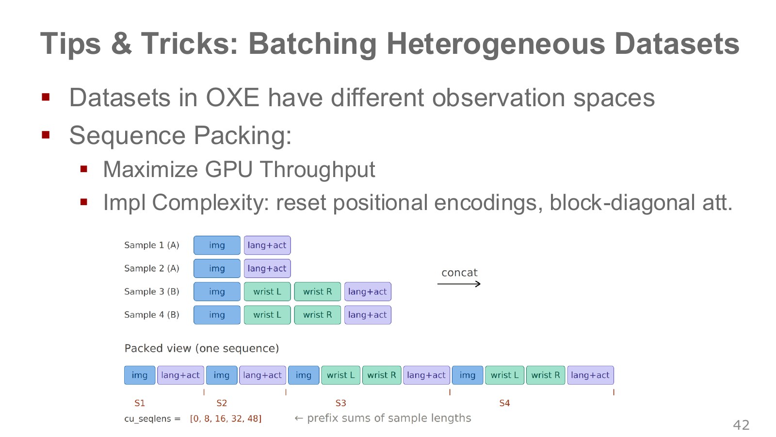
Concatenating variable-length samples within a batch reduces padding. Record each sample’s start and end to prevent unrelated images and instructions from mixing.

Original lecture, 40:36

#P044 · Blocking attention across sample boundaries

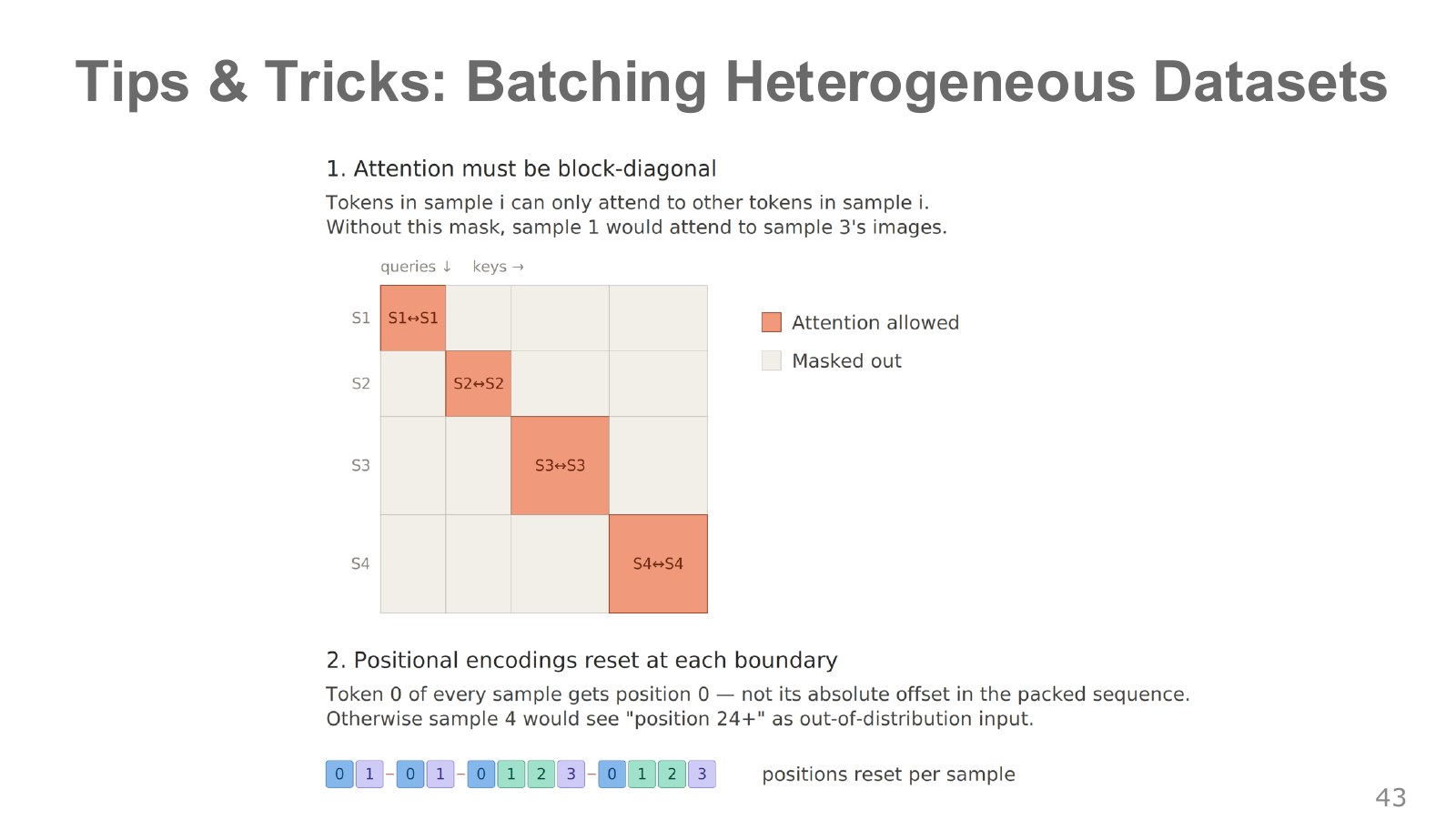
The diagonal blocks permit token references only within the same sample. Position indices restart for each sample too. Add causal constraints if the task also requires restricting temporal direction.

Concatenating lengths 3 and 5 gives boundaries 0, 3, and 8. Position indices are 0,1,2 for the first sample and restart at 0,1,2,3,4 for the second. Add a temporal causal mask if future actions must be hidden within each example. Packing must prevent examples from different homes and robots from leaking targets to one another.

Original lecture, 41:32

#P045 · Reading throughput and mixing quality

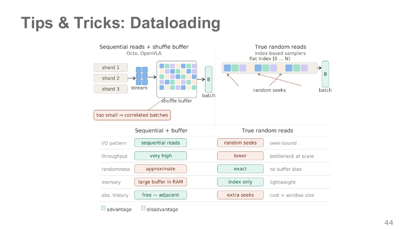
Sequential reads suit storage devices, but a small buffer can crowd batches with neighboring frames from one demonstration. Random reads improve mixing while increasing storage seeks. Measure both throughput and embodiment/task proportions within batches when choosing a strategy.

Mees recalls poor generalization in early Octo runs using a roughly 20,000-sample buffer and trajectory-level shuffling. The team mixed frames across trajectories before image decoding and expanded the buffer to about 500,000 samples. Since both changes were introduced together, the result cannot be attributed solely to buffer size.

A shuffle buffer temporarily stores streamed data for random sampling. If one long demonstration fills most of it, different batches may repeatedly see almost the same table and arm poses. Large buffers of decoded images are expensive, so mixing compressed frames first and decoding only sampled images can help.

Building a full-dataset index and reading randomly provides direct access across the dataset. Slow seeks and small-file reads can leave GPUs waiting for batches. A compromise randomly selects large chunks and shuffles within them. The data-loader experience shows that the sequence of experience reaching an unchanged model can affect outcomes.

Original lecture, 42:49

#P046 · Multiple output heads versus one action module

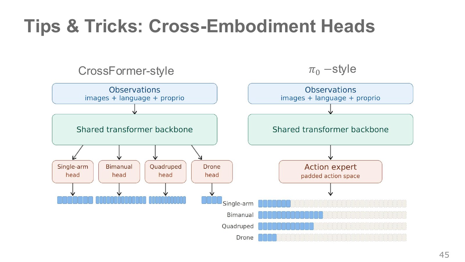
The left uses separate equipment-specific heads. The right uses one module outputting a common-length vector, with each embodiment selecting valid components. Equal vector lengths still require separately defined physical semantics per dimension.

Consider WidowX at 5 Hz and a dual-arm robot at 50 Hz. The same ten-step action chunk spans two seconds for the former and 0.2 seconds for the latter. Separate heads, as in CrossFormer, can specify different action dimensions and chunk lengths. A shared action module requires a maximum-size vector, valid-dimension masks, and equipment-specific mappings. Always examine chunk length alongside its physical time horizon.

Original lecture, 46:07

#P047 · How does the model identify the embodiment?

The same photograph and instruction may require different commands for different connected arms. Embodiment can be specified explicitly or inferred from joint states and images.

Original lecture, 48:18

#P048 · Specify equipment or infer it from observations

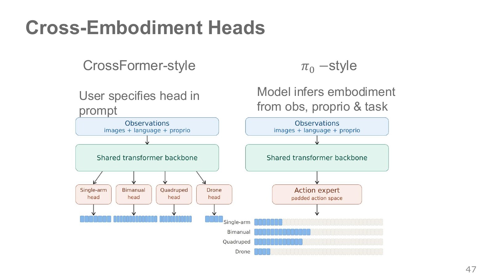
The left selects the specified embodiment’s head. In the single-expert design on the right, images, proprioceptive states, and task instructions provide equipment clues. Whether these clues produce correct outputs on unfamiliar hardware needs separate evaluation.

Original lecture, 48:52

#P049 · Joint learning with FAST tokens and continuous actions

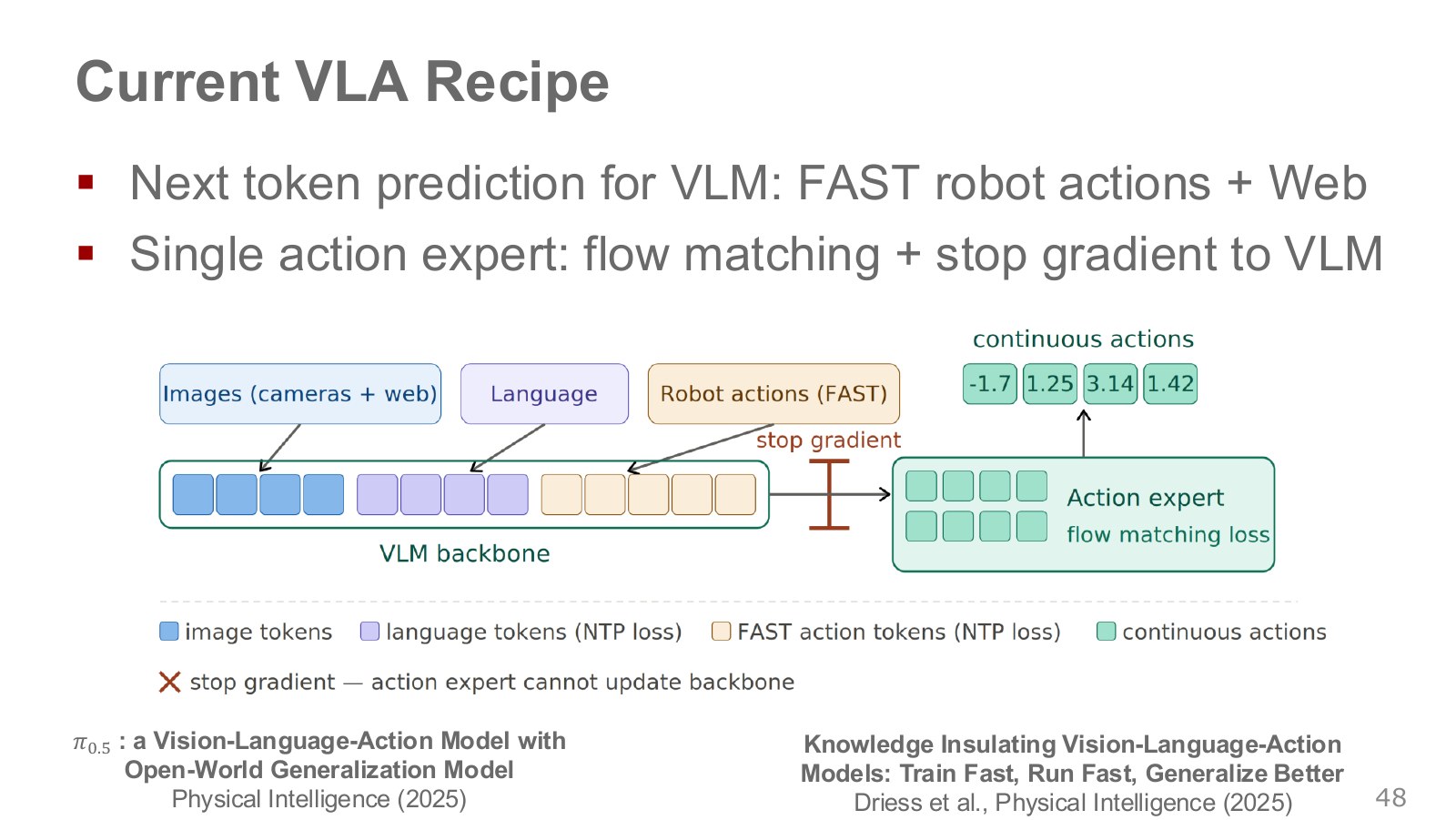
FAST supplies supervision through tokens compressing motion across time. A continuous action module uses flow matching to generate executable numerical chunks, while a stopped-gradient path prevents its loss from directly changing the backbone. Token and web-data losses still train the backbone. Knowledge Insulation

The paper’s action expert reads VLM observation representations but not the ground-truth FAST action tokens used as training targets. Reference restrictions and gradient blocking serve different roles: one controls information available for prediction; the other controls which parameters a continuous-action loss updates. Research team’s explanation

Read gradient insulation as two training paths. The backbone reads images and instructions and learns through FAST action-token and web-text prediction losses. The action expert reads backbone features and learns to predict continuous action chunks. Web cotraining helps preserve semantic representations, while the separated gradient path restricts how action learning changes the backbone. Sharing representations differs from letting every loss update every layer.

Original lecture, 52:06

#Comparing simulation scores with physical robots

#P050 · Repeat evaluation across environments too

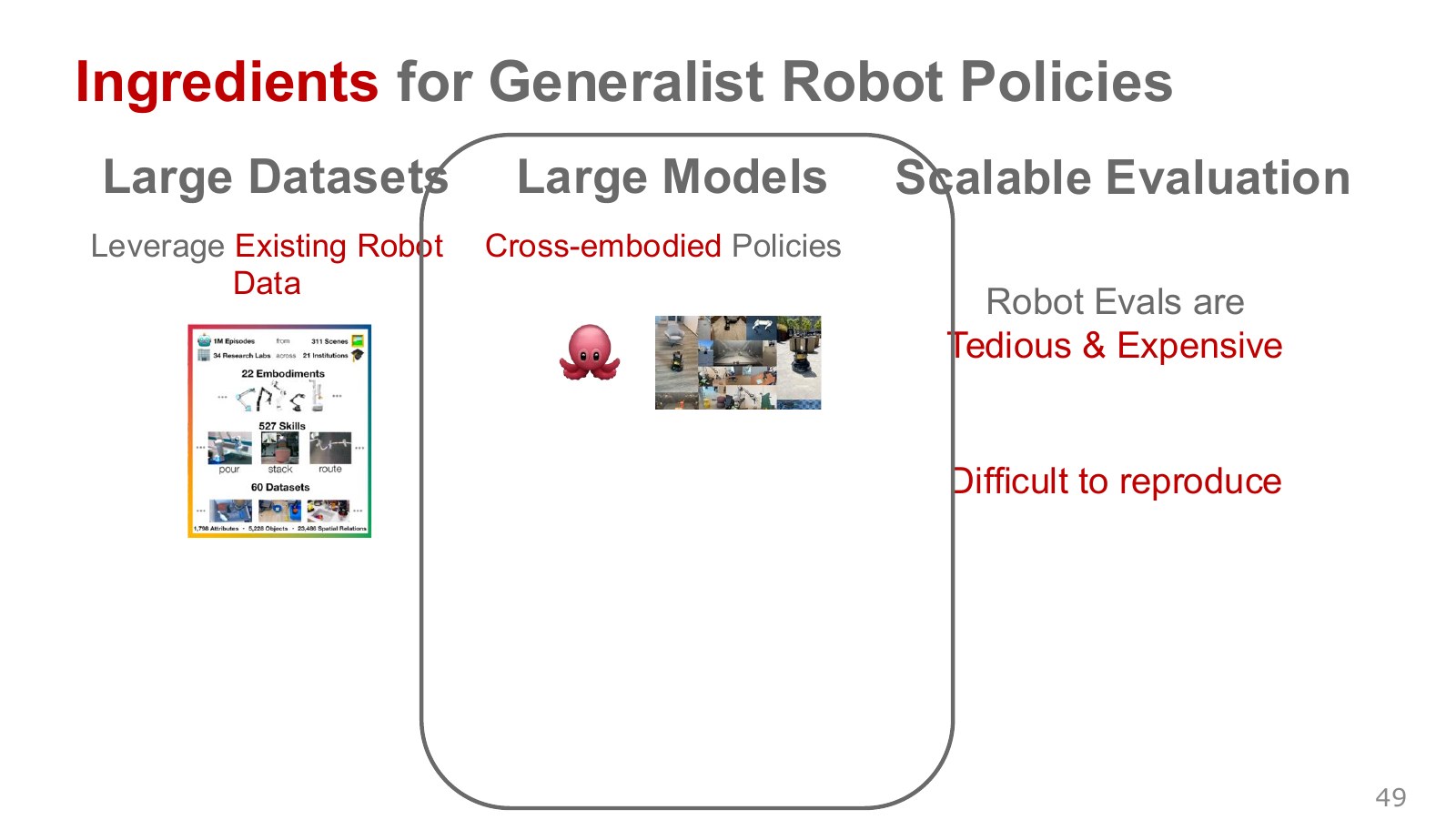
Scaling data and models also expands the evaluation fleet. Beyond a few illustrative videos, vary object positions or backgrounds and repeat matched conditions to make comparisons.

Original lecture, 54:10

#P051 · Changing conditions in physical evaluation

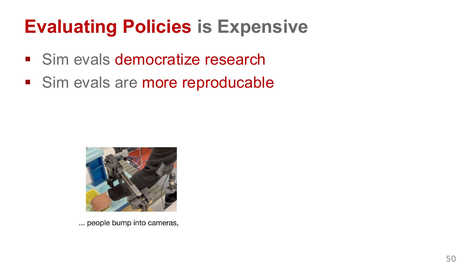
A bumped camera or shifted object can change results from the same checkpoint. Simulation makes initial conditions easier to repeat; real evaluation captures actual contact and friction.

Another lecture example replaces a broken motor. Changed joint zeros or sensor readings can make a policy interpret the same arm pose differently. As with camera shifts, record hardware settings and calibration before interpreting checkpoint comparisons.

Original lecture, 54:50

#P052 · Recreating physical evaluation environments in simulation

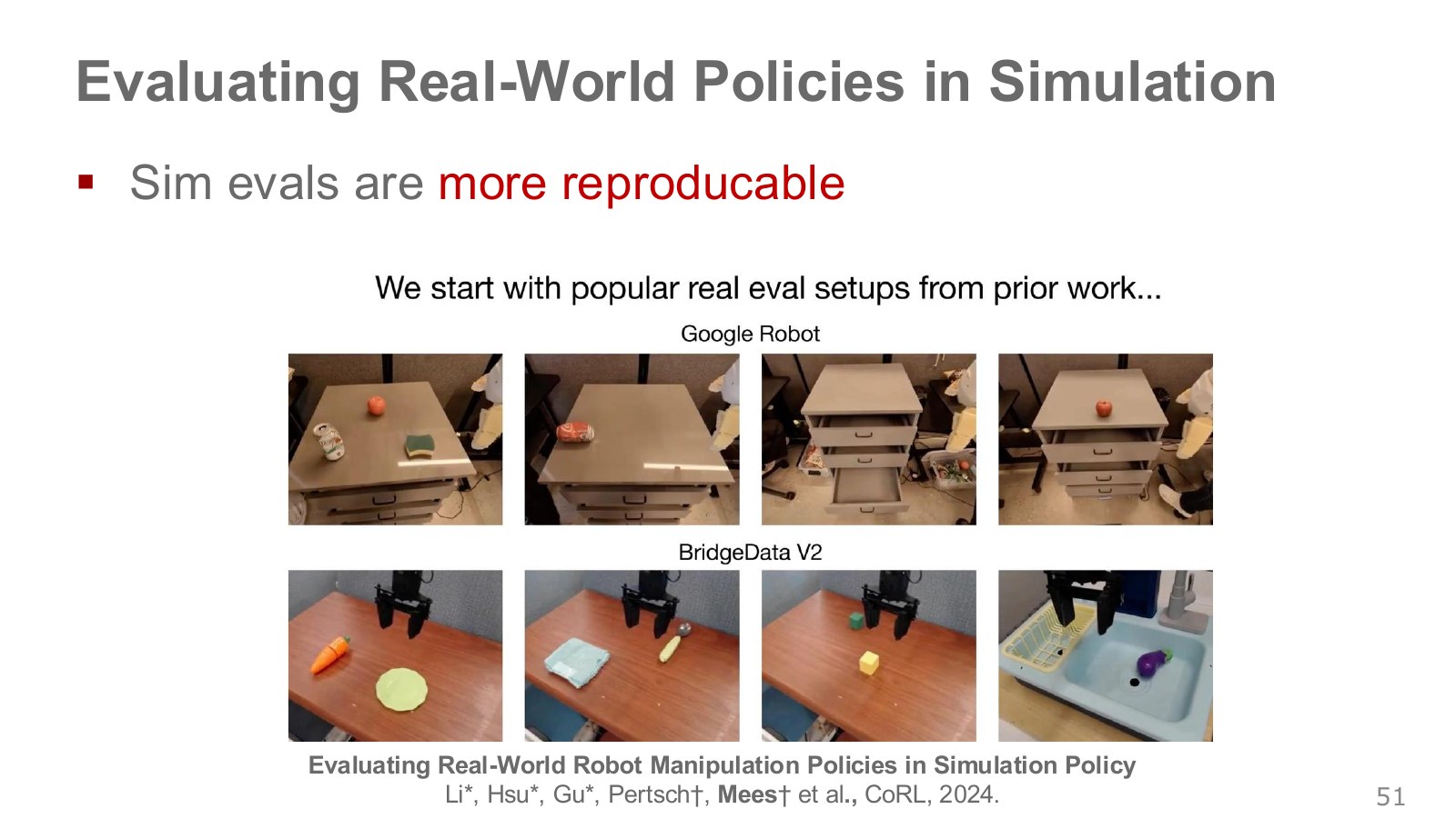
SIMPLER matches existing Google Robot and WidowX evaluation scenes. Running policies under corresponding instructions still requires examining effects of camera and controller mismatches. SIMPLER project

Original lecture, 56:52

#P053 · When relative rankings matter more than absolute success rates

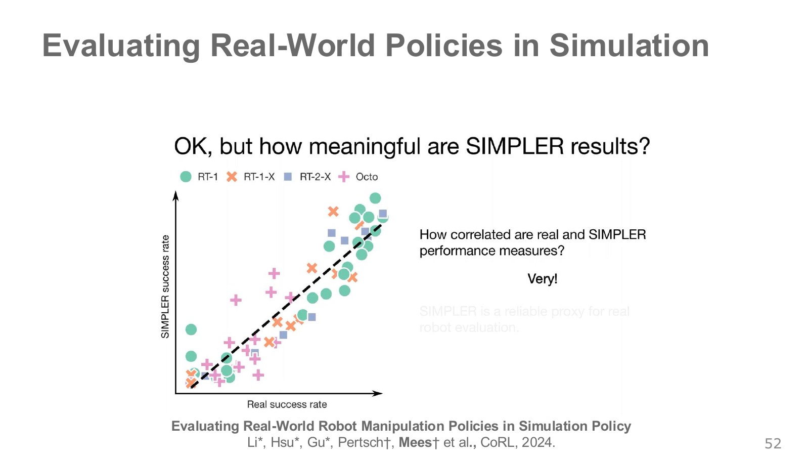
Each scatter point links real and simulated results for the same policy and task. Similar rankings can help shortlist candidates, but ranking transfer to new tasks and actual success rates require real-world verification.

For example, simulation might give A 70% and B 50%, while reality gives A 55% and B 40%. The numbers differ but A still outranks B. If new friction conditions reverse the ranking, simulation-based selection needs reevaluation there. Repeat policies from matched initial arrangements and check corresponding real tasks. These percentages illustrate rank correlation rather than report experimental measurements.

Original lecture, 58:10

#P054 · Compare end-effector paths under identical commands

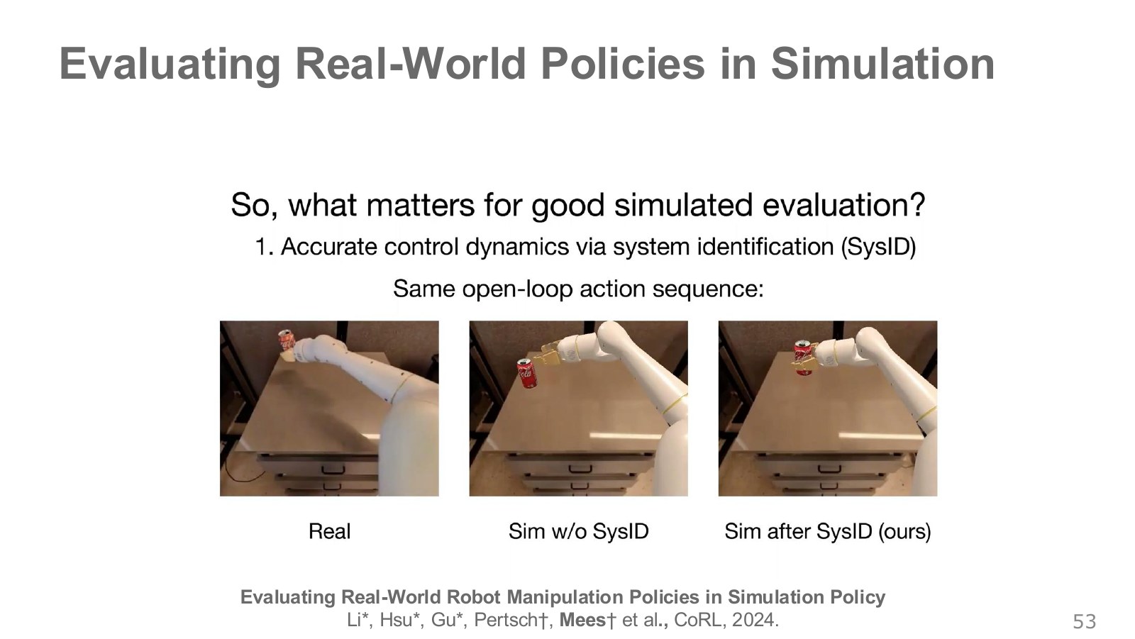
Feed identical command sequences to hardware and simulation and compare end-effector trajectories. Adjusting the control response to reduce their mismatch is system identification. Read the before-and-after paths as discrepancies between commands and resulting movement.

Original lecture, 59:02

#P055 · Match what the camera sees too

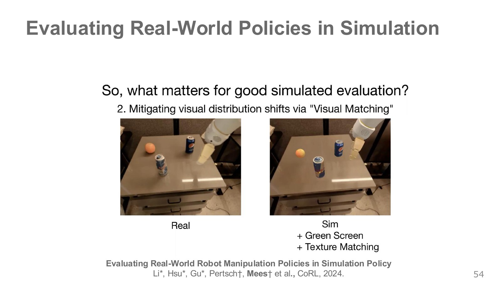
Background and texture differences between physical and virtual workbenches change policy inputs. Visual Matching reduces appearance mismatch to focus control comparisons. Contacts and joint delays instead concern the preceding slide’s dynamics.

The green-screen approach separates simulated moving robots and objects and composites them onto real workbench backgrounds. Texture matching applies real can patterns to virtual cans. The first primarily changes backgrounds; the second object appearance. SIMPLER project

Original lecture, 59:40

#P056 · Directions for later benchmarks

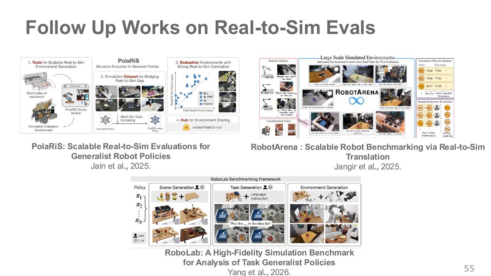
PolaRiS, RobotArena, and RoboLab expand comparisons by transferring physical scenes into varied virtual environments. Compare supported equipment, cameras, tasks, and paired real/simulated experiments first.

Original lecture, 61:39

#P057 · Connecting training and evaluation

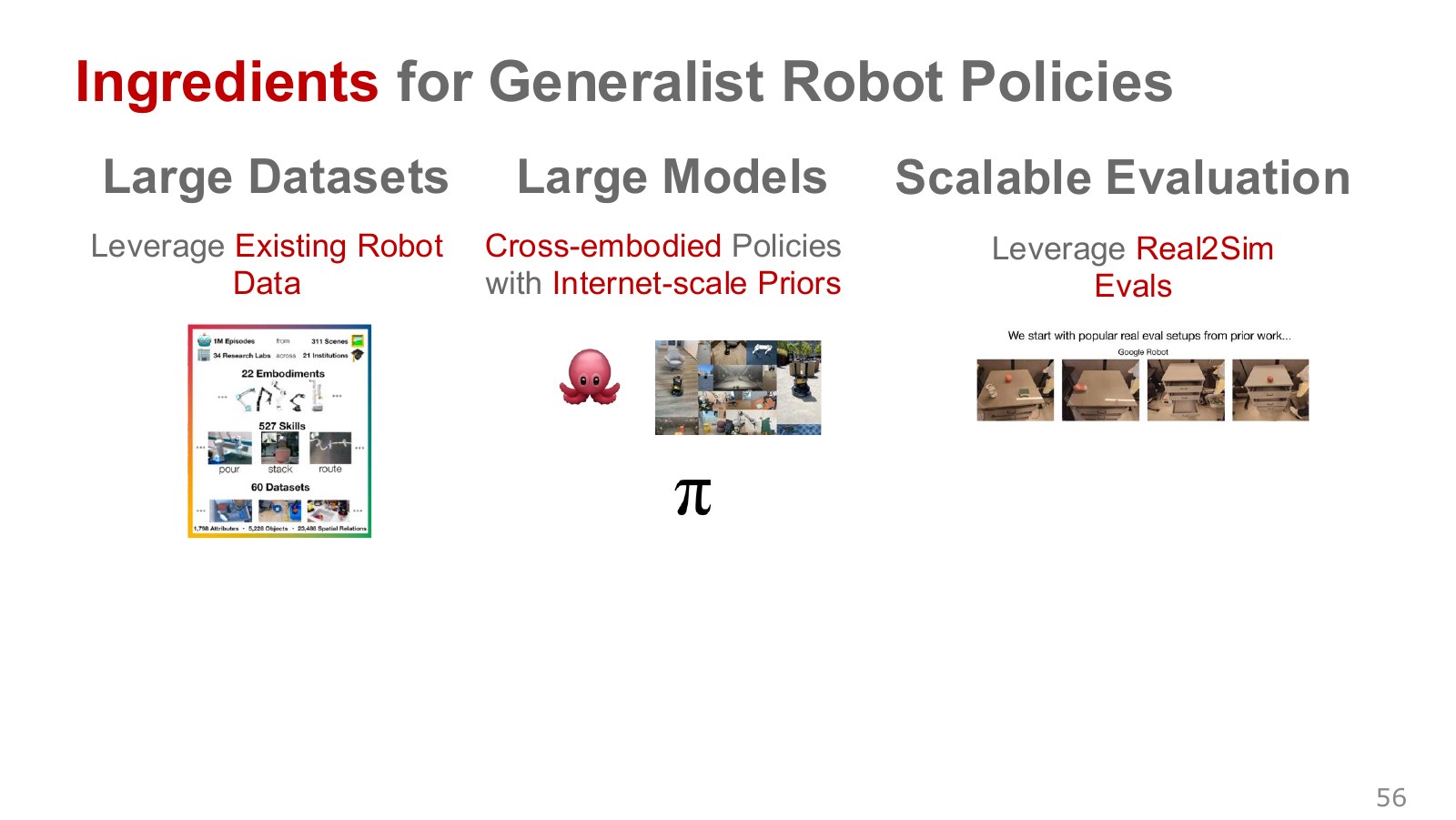
Even one grasping task requires aligning gripper semantics in data, connecting embodiment-specific outputs in models, and separately testing new objects and new hardware. Recording choices across all three stages helps locate the next failure.

Original lecture, 62:25

#Success rate and execution time in the invited talk

Quan Vuong compares success and execution time for the same tasks. Two policies may each succeed eight times out of ten, yet one takes thirty seconds and the other fifteen, changing throughput. The graph’s horizontal axis is execution time and its vertical axis success rate. These figures illustrate reading the axes, rather than quote measurements. Quan Vuong’s invited talk, 3:43

Gato, an official reading, combines different observations and actions into sequences. RECAP in the π∗0.6 paper reuses experience from execution and human corrections to improve policies. Even the same pretrained policy changes according to which subsequent experiences are collected and used. Gato · π∗0.6 and RECAP