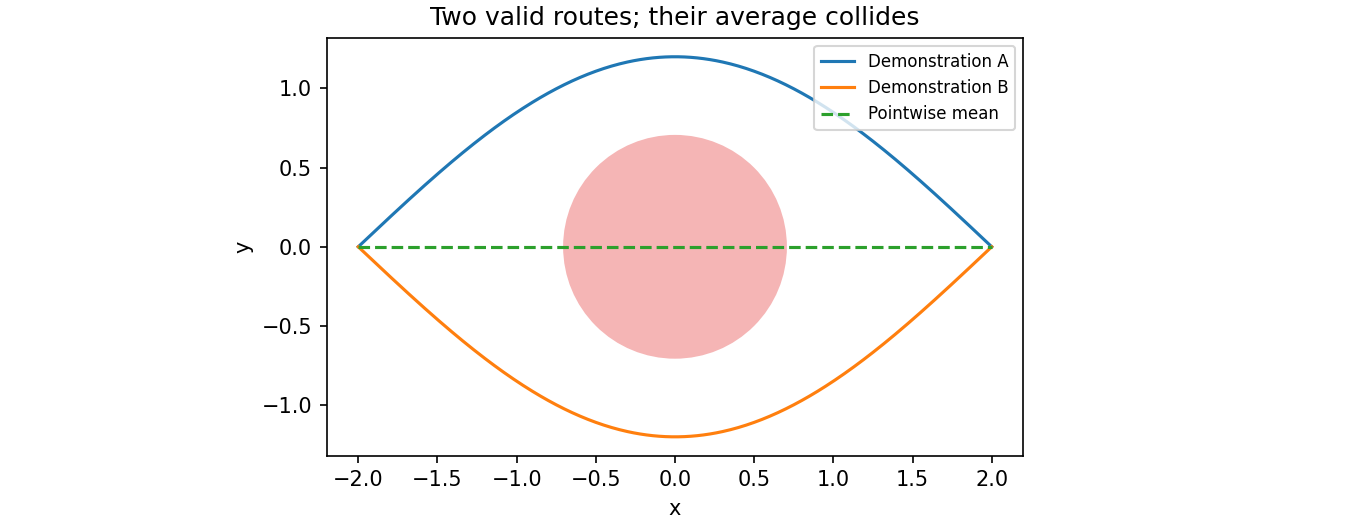
Going around an obstacle on either side can succeed. Yet averaging the two demonstrations sends the robot straight into it. This chapter explores how to generate executable actions without collapsing several valid answers into one.
Oier Mees · ETH Zurich 2026, Lecture 6 · Official lecture · Original PDF
#P001 · Learning a distribution of possible actions rather than a single average
Chapter 05 introduced policy gradients that increase the probability of good actions. Here, we focus on the shape of the distribution the policy can represent. Algorithms for improving policies and models for representing action distributions are different design choices. Generating actions with a diffusion model does not, by itself, constitute reinforcement learning.
A generative model learns a data distribution and produces new samples. It might generate photographs, or generate a sequence of future joint targets conditioned on camera observations and instructions. We consider latent-variable models, diffusion models, and flow matching in turn. The original course is called Robot Learning, and the main robot examples in this chapter use imitation learning from demonstrations.
#P002 · Opening the same drawer allows different joint configurations and approaches
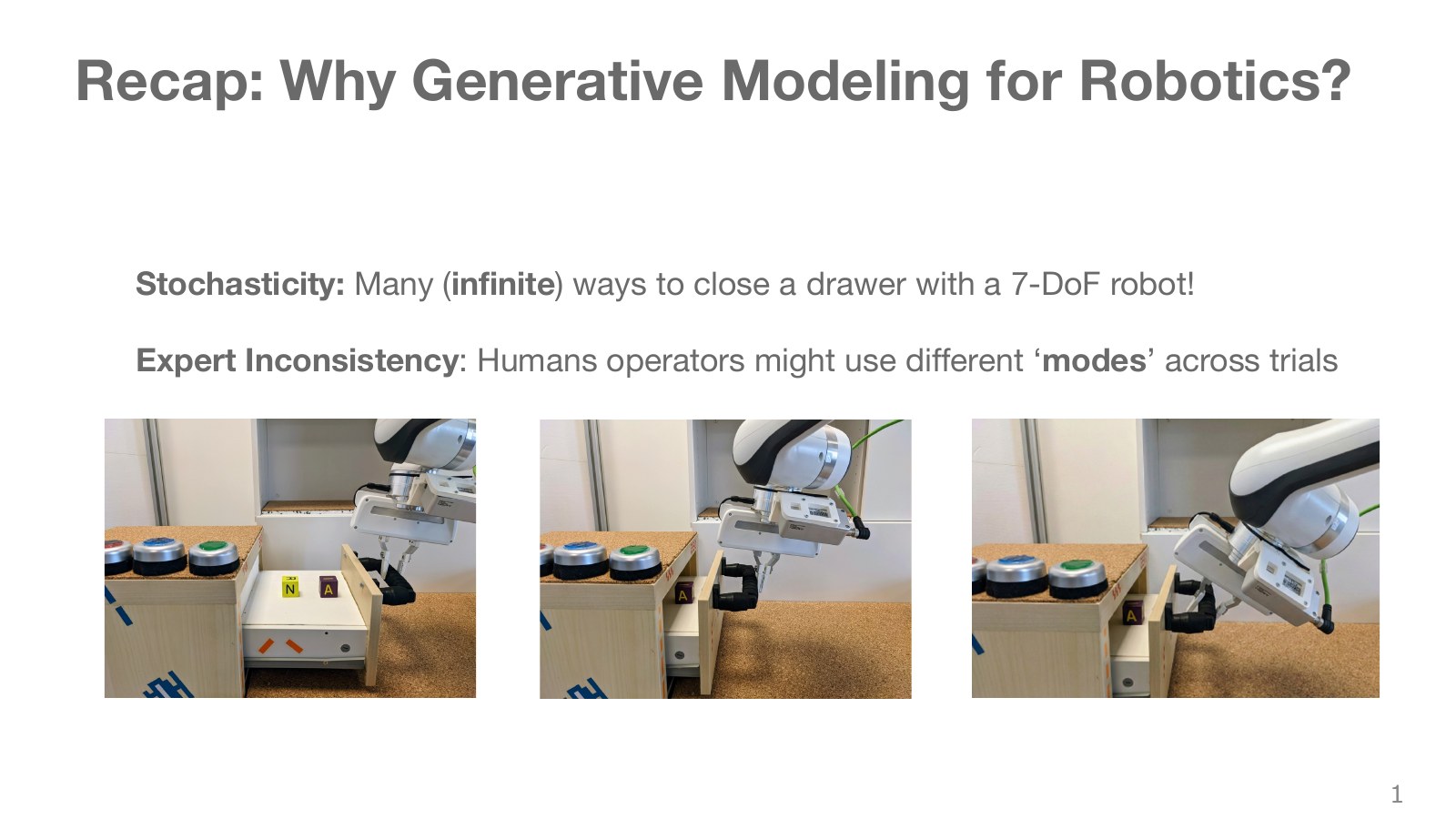
The robot arms in the three photographs adopt different configurations for the same drawer-opening goal. Different grasp positions, elbow orientations, and approach paths can all succeed. A seven-degree-of-freedom arm can move its elbow while maintaining the hand’s position and orientation. This kinematic redundancy means multiple configurations can achieve the same goal.
Demonstrators’ habits introduce further variation into the data. A regression model assuming one correct action per observation can miss these alternatives. Redundancy does not itself imply randomness: a deterministic policy can consistently choose one solution. A generative policy’s advantage is representing the distribution of several valid strategies together.
#P003 · Averaging left and right detours is not a safe compromise
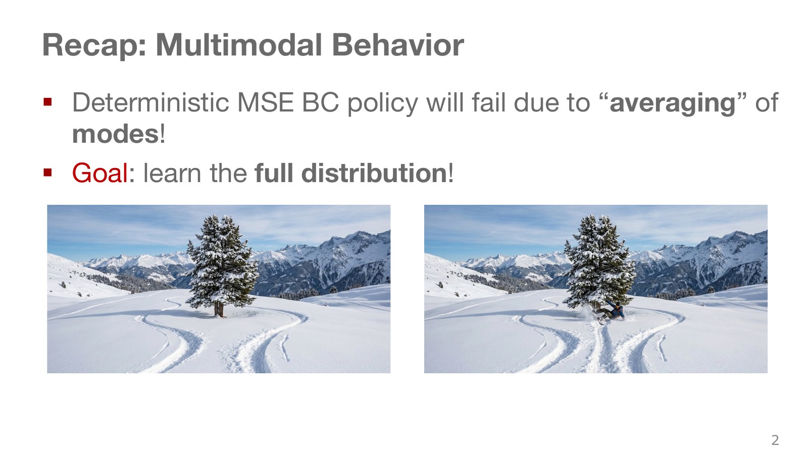
Consider the two paths around the tree in the middle. Both the left and right paths succeed, but averaging their positions at corresponding stages points toward the tree. Here, multimodality means multiple peaks in probability density. This differs from multimodal inputs such as cameras and language.
With sufficient expressive capacity and suitable training conditions, predicting one action by minimizing squared error targets the conditional mean action given the observation. If the region between two strategies is successful, averaging can work; if an obstacle lies between them, it becomes a problem. The precise point is not that averages are always bad, but that the average of separated valid answers is not guaranteed to be valid.
Explore the symbols and calculation The conditional mean targeted by squared-error regression
Read the equation in words
A single prediction minimizing squared error is the conditional mean of possible answers for the same observation. Averaging different action strategies can produce a poor action.
Understand each symbol
- The action chosen at step : for example, a torque, a joint target or a movement direction, depending on the setup.
- The sensor observation at step . It is not assumed to equal the full physical state.
- The optimal single-action prediction under this loss.
- An expectation: an average over possible outcomes weighted by their probabilities.
- Conditional notation: the information to the right of the bar is given. This is not a division sign.
Follow the calculation
- Consider which actions can occur for the same observation.
- Average them according to their probabilities.
Check with a small example
If half the demonstrations go left at −1 and half right at +1, the mean is 0. Even if no demonstration uses 0, it is the optimal single squared-error prediction.
An illustrative example for understanding the equation.
#P004 · Three starting points for modeling complex action distributions
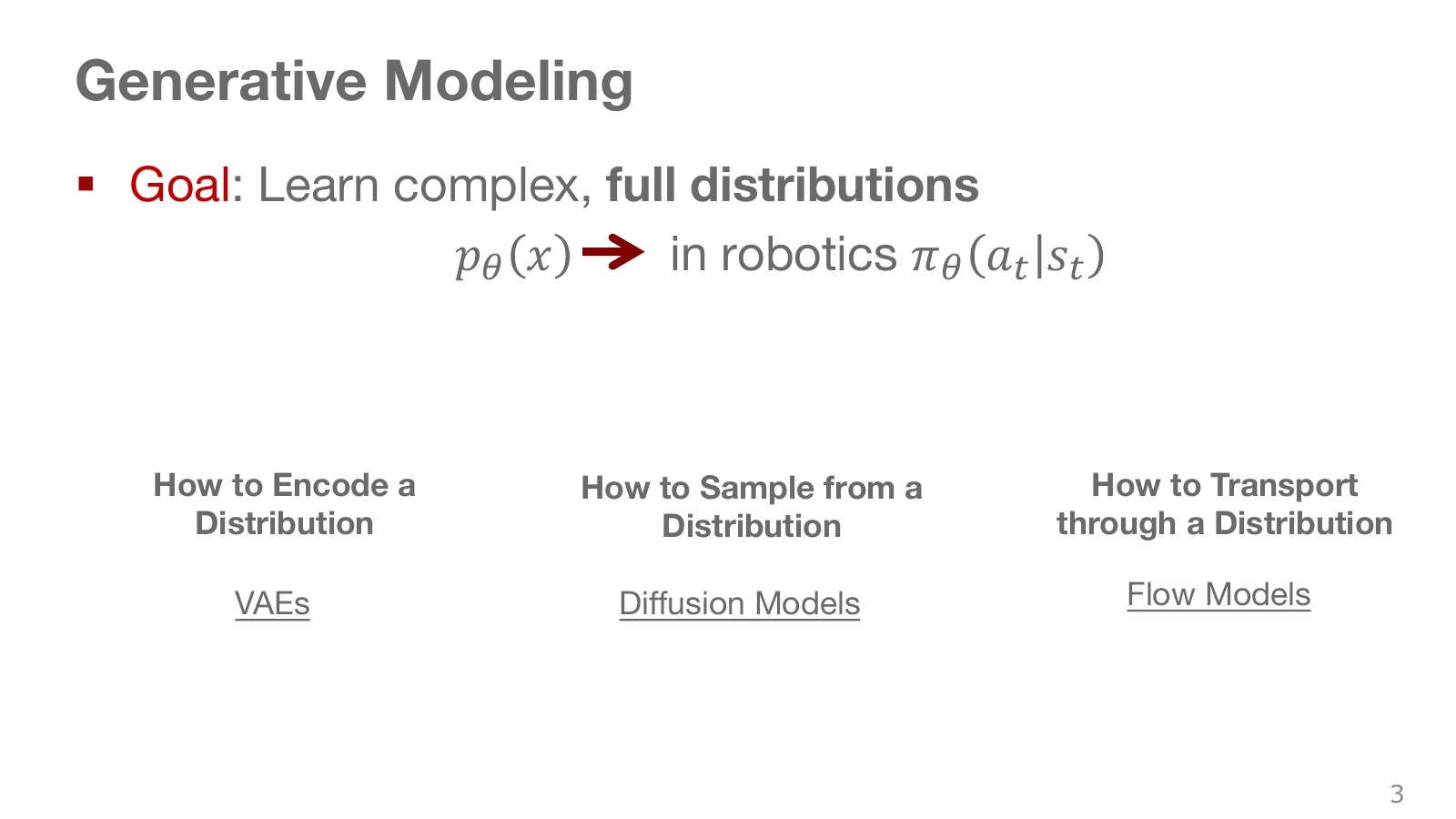
The latent-variable model on the left generates complex outcomes from a simple hidden variable. The diffusion model in the middle learns to reverse the addition of noise to data. Flow matching on the right learns a vector field transporting noise samples into the data distribution. All three begin with easily sampled random inputs to represent complex distributions.
For robot applications, condition these models on current images, joint states, and task instructions. The aim is not to generate arbitrary actions but actions that open this drawer in this scene. These three families do not exhaust generative modeling: autoregressive models and GANs also exist. The lecture focuses on three families leading to robot action generation.
#P005 · What it means to generate a sample from noise
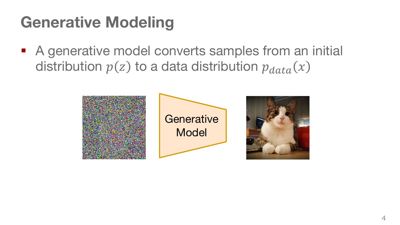
The figure starts with a vector of numbers sampled from a normal distribution and ends with a cat image. A normal distribution concentrates values in a bell shape around its mean; the standard normal has mean zero and variance one along each axis. A network learns a transformation from random numbers into outputs resembling the data.
Do not understand this solely as memorizing a particular cat photograph assigned to every noise vector. The learning principle should make the overall distribution of transformed samples resemble the data distribution. For robots, output numbers can represent joint targets or hand displacements instead of pixel intensities. Even with the same random input, different observation conditions should produce different actions.
#P006 · A latent variable captures choices among action strategies
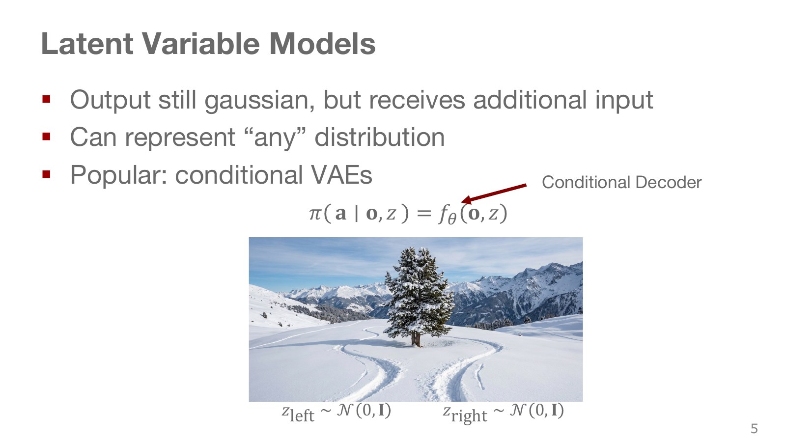
A latent variable is not directly given in the data but explains differences in outcomes. Think of approaching a cup from the left or right as a hidden choice. First sample the latent variable, then generate an action from both the observation and that variable.
Explore the symbols and calculation A conditional action distribution obtained by averaging over latent variables
Read the equation in words
Create a different action distribution for each latent value, then combine all latent possibilities into the overall action distribution for the observation.
Understand each symbol
- The action chosen at step : for example, a torque, a joint target or a movement direction, depending on the setup.
- The sensor observation at step . It is not assumed to equal the full physical state.
- A latent vector representing factors such as execution style that the model does not directly observe. It is sampled or inferred by an encoder.
- The prior distribution of latent values before observing the data.
- The parameters collecting the trainable weights of the network or policy.
- Conditional notation: the information to the right of the bar is given. This is not a division sign.
Follow the calculation
- Calculate action likelihood conditioned on each latent value.
- Weight by the latent prior and integrate across latent space.
Check with a small example
With two equally likely discrete modes assigning an action likelihoods 0.8 and 0.2, the mixture likelihood is 0.5. For continuous latent values, this sum becomes an integral.
An illustrative example for understanding the equation.
The integral combines the distributions produced by different latent variables according to their frequency. Even if each conditional distribution is simple, the combined distribution can have several peaks. Distinguish expressive power available with sufficiently flexible networks and latent spaces from performance actually learned from limited data.
Within an action sequence, maintaining the chosen strategy matters. Independently switching between left and right at every control instant can make the hand oscillate. Matching the distribution and producing temporally consistent behavior must be considered together.
#P007 · An autoencoder reconstructs inputs from compressed information
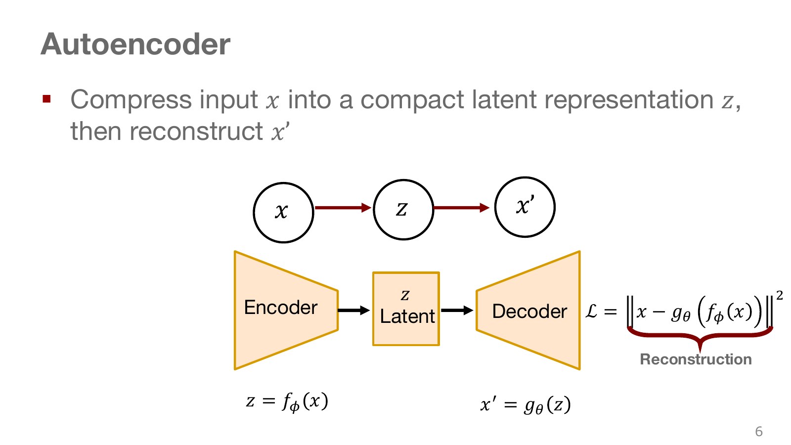
The encoder on the left compresses a large input into a smaller vector; the decoder on the right reconstructs the input from that vector. For photographs, a representation smaller than the pixel array can capture information such as object shape and arrangement. Reconstruction means producing an output resembling the input.
Explore the symbols and calculation Autoencoder encoding, reconstruction, and loss
Read the equation in words
Compress an input into a small representation, reconstruct the original, and learn from squared reconstruction differences.
Understand each symbol
- A latent vector representing factors such as execution style that the model does not directly observe. It is sampled or inferred by an encoder.
- Weights of a different network. Read which model they belong to together with the calculation steps.
- The parameters collecting the trainable weights of the network or policy.
- The original input and its reconstruction estimate.
- Respectively, the encoder compressing the input and the decoder reconstructing it.
- The squared length obtained by squaring and summing all vector components. It combines coordinate-wise errors into one nonnegative quantity.
Follow the calculation
- The encoder transforms the input into a latent vector.
- Sum componentwise squared differences between the decoder reconstruction and original input.
Check with a small example
Input [1,3] and reconstruction [2,2] give reconstruction loss .
An illustrative example for understanding the equation.
Encoder weights are denoted by and decoder weights by . The bottleneck limits intermediate representation capacity. Too small a bottleneck loses needed information; too large a bottleneck may simply memorize inputs. Good reconstruction does not ensure preservation of contact or safety information essential to robot control. The inputs and reconstruction targets matter.
#P008 · Codes that support reconstruction are not necessarily codes we can sample usefully
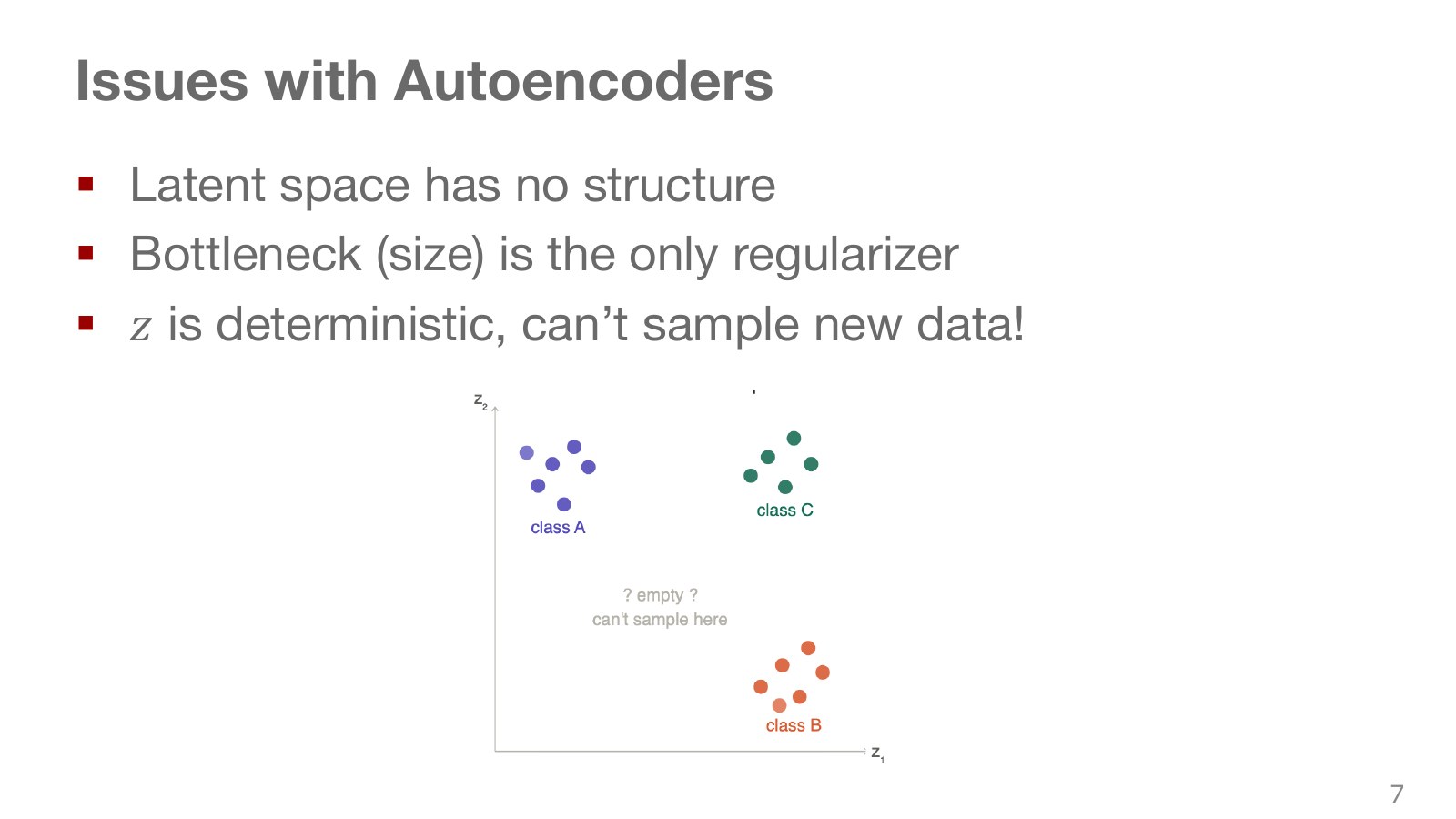
Consider the clusters of colors in latent space. An autoencoder may reconstruct well where training inputs map, yet learn little about the sparsely used areas between them. Sampling an arbitrary point from a standard normal and feeding it to the decoder therefore need not produce a good sample.
The decoder being deterministic is not itself the problem. A deterministic transformation of random input can still generate a probability distribution. The key limitation of an ordinary autoencoder is the lack of a mechanism aligning the distribution used to sample codes later with how the space is populated during training.
#P009 · A VAE learns reconstruction and latent-distribution regularity together
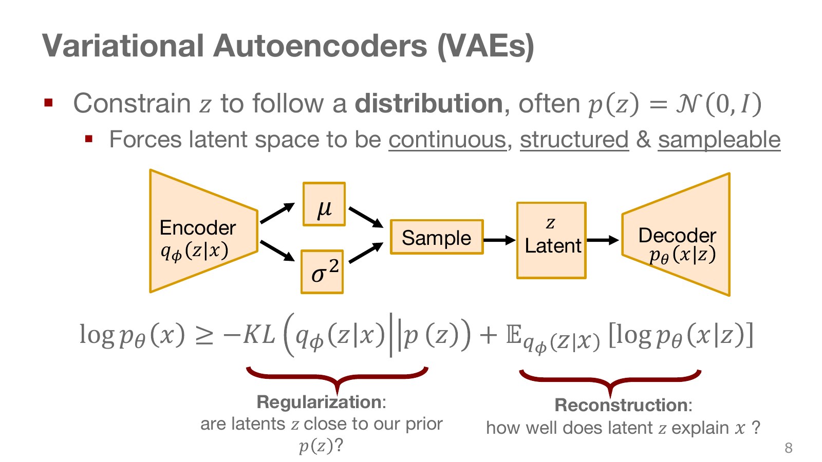
A variational autoencoder (VAE) encoder outputs a mean and variance rather than a single code. A code sampled from that distribution goes to the decoder. The prior specifies how to sample codes before observing data; the approximate posterior estimates suitable codes after seeing an input.
Explore the symbols and calculation Reconstruction and prior-regularization terms
Read the equation in words
This lower-bound objective explains reconstruction while preventing the encoder's latent distribution from moving too far from the prior. Larger values are better.
Understand each symbol
- The encoder, or approximate posterior, estimating a latent distribution after seeing the input.
- The decoder describing a distribution over original data given a latent value.
- The prior distribution of latent values before observing the data.
- KL divergence comparing two distributions. It is nonnegative and generally changes when the direction is reversed.
- A lower bound on data log likelihood, maximized during training.
- An expectation: an average over possible outcomes weighted by their probabilities.
- The natural logarithm. It converts products into sums and is defined only for positive inputs.
- Conditional notation: the information to the right of the bar is given. This is not a division sign.
Follow the calculation
- Average reconstruction log likelihood over latent values proposed by the encoder.
- Subtract KL between the encoder distribution and prior to balance the objective.
Check with a small example
A reconstruction term of −2 and KL of 0.5 give ELBO −2.5. Negate it to construct a minimization loss.
An illustrative example for understanding the equation.
Explore the symbols and calculation Why the ELBO is a lower bound on log likelihood
Read the equation in words
The gap between the ELBO and actual log likelihood is KL between the approximate and true posteriors. This nonnegative gap prevents the bound from exceeding the actual value.
Understand each symbol
- A latent vector representing factors such as execution style that the model does not directly observe. It is sampled or inferred by an encoder.
- The encoder, or approximate posterior, estimating a latent distribution after seeing the input.
- KL divergence comparing two distributions. It is nonnegative and generally changes when the direction is reversed.
- The true posterior over latent values after observing data, distinct from the prior.
- The natural logarithm. It converts products into sums and is defined only for positive inputs.
- Conditional notation: the information to the right of the bar is given. This is not a division sign.
Follow the calculation
- Subtract the lower bound from full log likelihood to identify the remaining distribution mismatch.
- The gap is zero when the approximate posterior equals the true posterior.
Check with a small example
Actual log likelihood −1 and lower bound −1.4 give a KL gap of 0.4.
An illustrative example for understanding the equation.
The expectation in the first equation evaluates how well a sampled code explains the input. KL divergence is a nonnegative measure of distribution mismatch. Since the second equation’s KL is nonnegative, the ELBO cannot exceed log likelihood. Its name, evidence lower bound, describes precisely this lower bound on observed-data log likelihood. Distinguish the KL against the prior from the KL against the true posterior measuring the bound’s gap.
Berkeley’s VAE lecture, 53:50–56:53 explains the source of this gap. The equation relates increasing the bound to increasing actual likelihood. A conditional action model can use an encoder seeing observations and demonstrated actions, and a decoder reconstructing actions from observations and latent variables. At execution time, future demonstrated actions are unknown and cannot be supplied as answers to the training encoder.
#P010 · Reparameterization creates a gradient path while retaining randomness
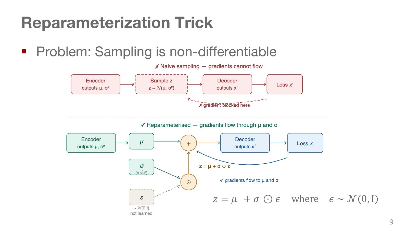
Leaving the distribution-sampling operation unchanged makes derivatives through to encoder weights inconvenient. Instead, draw standard-normal noise separately and transform it using the mean and standard deviation.
Explore the symbols and calculation Reparameterizing a Gaussian latent variable
Read the equation in words
Transform standard noise using an input-dependent mean and standard deviation to obtain a latent sample. Keep randomness in the noise and differentiate the learnable transformation.
Understand each symbol
- Sample a Gaussian noise vector with component means 0 and variances 1.
- Weights of a different network. Read which model they belong to together with the calculation steps.
- The latent distribution's mean and standard deviation output by the encoder.
- The symbol for elementwise multiplication.
Follow the calculation
- The encoder calculates the latent mean and standard deviation.
- Multiply noise by standard deviation elementwise and add the mean.
Check with a small example
Mean 2, standard deviation 0.5, and noise −1 give latent sample 1.5. If variance is 0.25, the multiplier is standard deviation 0.5, not variance 0.25.
An illustrative example for understanding the equation.
The multiplication symbol in the middle means elementwise multiplication. For one backpropagation pass, hold the sampled noise fixed and differentiate how reconstruction changes with the mean and standard deviation. Randomness is not removed; its source is moved outside the weights.
Also distinguish variance from standard deviation. If the figure’s denotes variance, its square root belongs in the equation above. If an implementation outputs log variance, halve it and exponentiate to obtain standard deviation. Chapter 05’s SAC uses the same pathwise-derivative idea for action samples.
#P011 · Differentiating probabilities versus the path that generates samples
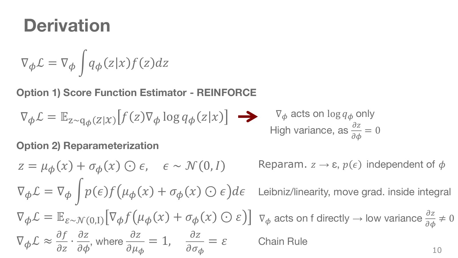
The left side shows the score-function approach, calculating how outcome weights change as a distribution changes. REINFORCE’s log-probability derivative belongs here. The right side shows the pathwise approach, differentiating directly through the function generating an outcome from fixed noise.
Explore the symbols and calculation Pathwise derivatives through differentiable reparameterization
Read the equation in words
Instead of differentiating a direct distribution-sampling operation, follow the path transforming independent noise through a differentiable function.
Understand each symbol
- Weights of a different network. Read which model they belong to together with the calculation steps.
- A latent vector representing factors such as execution style that the model does not directly observe. It is sampled or inferred by an encoder.
- A differentiable transformation from noise to a latent sample.
- The objective function evaluated at the latent sample.
- An expectation: an average over possible outcomes weighted by their probabilities.
- A gradient collects componentwise derivatives describing how much the result changes when a variable changes.
Follow the calculation
- Express the sample as a function of weights and noise.
- Hold the noise fixed, differentiate the function's weight dependence, then average over noise.
Check with a small example
If the latent value is weight plus noise and the output function squares it, weight 1 and noise 0 give derivative 2. This method cannot be applied unchanged to every stochastic sampling operation.
An illustrative example for understanding the equation.
This expression requires a noise distribution independent of the weights and conditions permitting interchange of expectation and differentiation. Linearity of expectation alone does not make every random computation differentiable. Pathwise methods are useful for many continuous latent models, but do not universally guarantee lower variance or apply directly to discrete samples. They require a differentiable path to the output.
#P012 · Generation starts from the prior without a training input
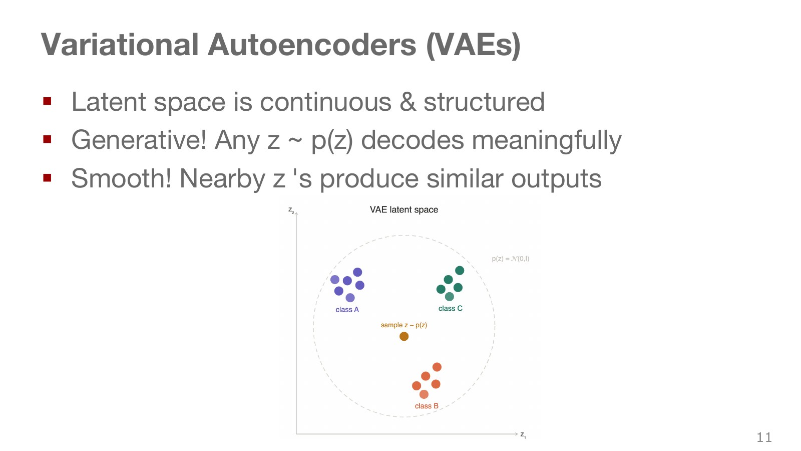
The upper part shows training, which passes an input through the encoder; the lower part shows generation, which samples a code from the prior and sends it to the decoder. A VAE aims to create a shared latent space connecting these processes. Similar codes yielding similar outputs can help interpolation and sampling.
KL regularization does not guarantee that every code is meaningful or every intermediate output natural. In particular, whether interpolation between action codes produces collision-free motion requires separate checks against the physical environment and constraints. Latent-space smoothness and real-robot trajectory safety are different properties.
#P013 · The model may ignore latent variables or mismatch the prior
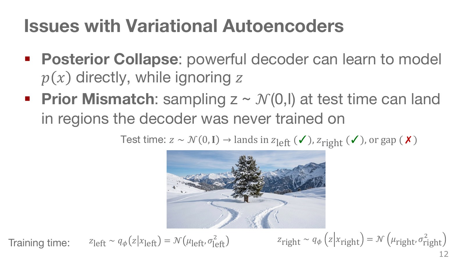
Posterior collapse occurs when the decoder barely uses the latent variable. If other conditions already support good reconstruction, or regularization pressure is strong, different codes may yield little variation. This does not necessarily make the decoder deterministic: it can have other sources of randomness.
Prior mismatch is a difference between the latent distribution actually used by training inputs and the prior sampled during generation. Think of aggregating the approximate posteriors across all inputs. A standard-normal sample landing in a region rarely used during training can reconstruct poorly. Low Gaussian density and being mathematically outside the support are different statements. Balancing reconstruction and regularization is a central VAE design issue.
#P014 · VQ-VAE replaces a continuous code with its nearest codebook entry
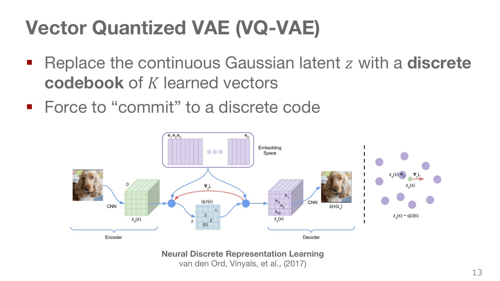
VQ stands for vector quantization. After the encoder produces a continuous vector, select the nearest representative from a fixed-size collection. The codebook is this list of representative vectors. The colored points denote codebook vectors, and each region contains inputs selecting the same representative.
Explore the symbols and calculation Selecting the nearest codebook entry
Read the equation in words
Find the codebook vector nearest the continuous encoder vector and replace the latter with that code. Subsequent stages can use finite code indices.
Understand each symbol
- The continuous vector produced by the encoder.
- The th codebook vector and total number of codes.
- The selected code index and its vector.
- The squared length obtained by squaring and summing all vector components. It combines coordinate-wise errors into one nonnegative quantity.
- Select the input attaining the largest or smallest value, rather than the value itself.
Follow the calculation
- Compute squared distances from the encoder vector to every codebook vector.
- Select the index with the smallest distance and retrieve its vector.
Check with a small example
For codebook [−1,1,3] and encoder output 0.7, select the nearest value, 1.
An illustrative example for understanding the equation.
The index is discrete, but the selected vector has real-valued components. “Code 7” and “a seven-dimensional vector” mean entirely different things. Codebook size and vector dimension are separate as well. Images can select codes by location and be represented by multiple tokens. Basic VQ-VAE training differs from a VAE that outputs Gaussian means and variances for each input and computes a KL term.
#P015 · Nearest-entry selection uses a surrogate gradient
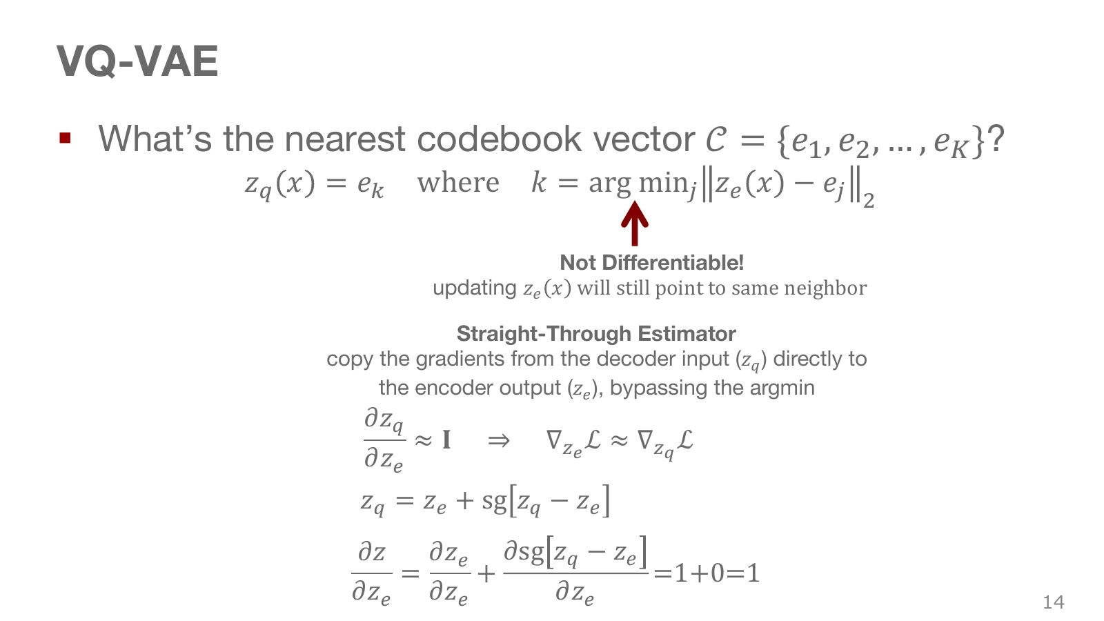
As the encoder output moves slightly, the quantized result stays unchanged while the same representative remains nearest. Its true derivative is therefore zero within that region and may be undefined at boundaries. Simply backpropagating reconstruction error through this operation would give the encoder an inadequate learning signal.
Explore the symbols and calculation A computational expression for the straight-through estimator
Read the equation in words
Use the quantized code forward, but pass an approximate gradient back to the encoder before quantization. This is not the exact derivative of true nearest-neighbor selection.
Understand each symbol
- The stop-gradient operation preserves the value while treating its derivative as zero.
- The encoder output, selected code, and straight-through expression.
Follow the calculation
- Adding the parenthesized difference during the forward pass leaves the quantized vector.
- During backpropagation, treat the stop-gradient term as constant and use only the encoder path.
Check with a small example
Encoder value 0.7 and code value 1 produce forward output 1. A nonzero surrogate gradient is nevertheless passed to the encoder despite discontinuous code-selection boundaries.
An illustrative example for understanding the equation.
Stop-gradient passes a value unchanged in the forward calculation but treats that path’s gradient as zero during backpropagation. The expression above outputs the quantized code forward and passes gradients to the encoder output as if through an identity. The STE is a surrogate gradient for learning, not the exact derivative of quantization. It permits training through discrete choices but should not be claimed to be unbiased.
#P016 · Reconstruction, codebook, and commitment terms update different components
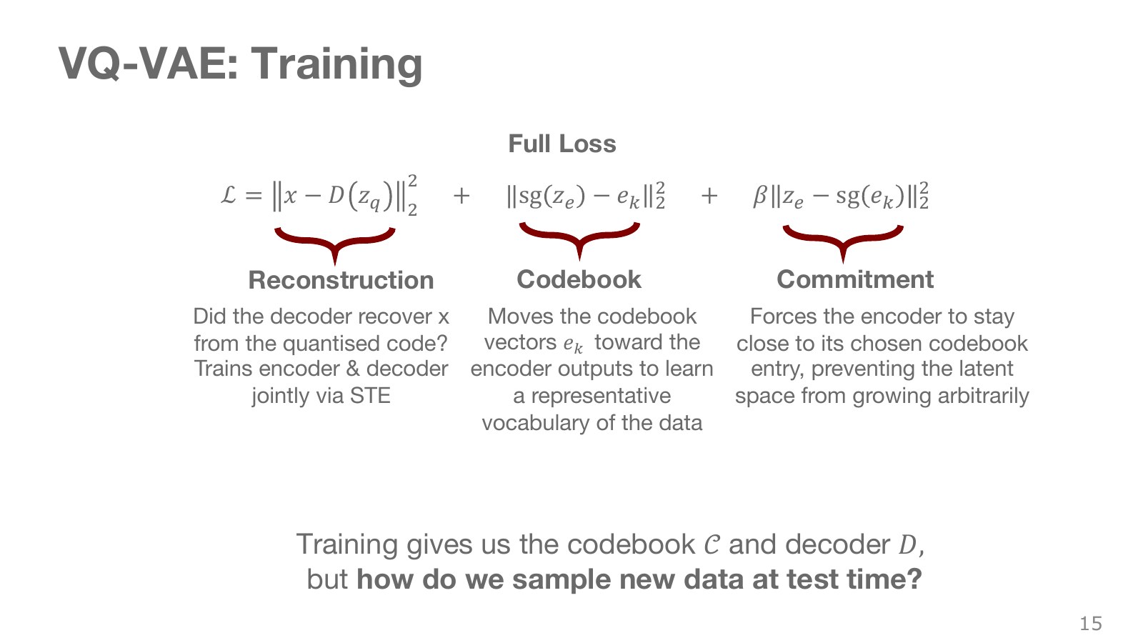
Separating the three losses reveals what each learns. Reconstruction recovers the original input from the code. The codebook term pulls the selected representative toward the encoder output. The commitment term keeps the encoder near its chosen representative.
Explore the symbols and calculation The three VQ-VAE training terms
Read the equation in words
Separate reconstruction, codebook movement, and encoder commitment into distinct training terms. Stop-gradient placement determines which weights each term changes.
Understand each symbol
- The original input and its reconstruction from the selected code.
- The encoder output and selected codebook vector.
- The commitment weight keeping the encoder near its code, distinct from diffusion noise variance later.
- An indication that this term does not pass derivatives to that variable.
- The squared length obtained by squaring and summing all vector components. It combines coordinate-wise errors into one nonnegative quantity.
Follow the calculation
- Reconstruction error trains the decoder and reaches the encoder through the STE.
- The second term moves the codebook toward encoder outputs; the third moves the encoder toward selected codes.
Check with a small example
Encoder value 0.7 and code value 1 have squared difference 0.09. A third-term weight of 0.25 gives that term value 0.0225.
An illustrative example for understanding the equation.
The middle term holds the encoder side fixed and changes the codebook. The last term holds the codebook side fixed and changes the encoder. Reconstruction error directly trains the decoder and reaches the encoder through the STE. Here, weights commitment; its role differs from the noise-variance symbol used later for diffusion.
A learned codebook alone does not determine which index combinations to sample or how often. That question leads to the next generation stage. Variants can also update codebooks through moving averages rather than direct loss gradients.
#P017 · Generating new codes also requires learning their index distribution
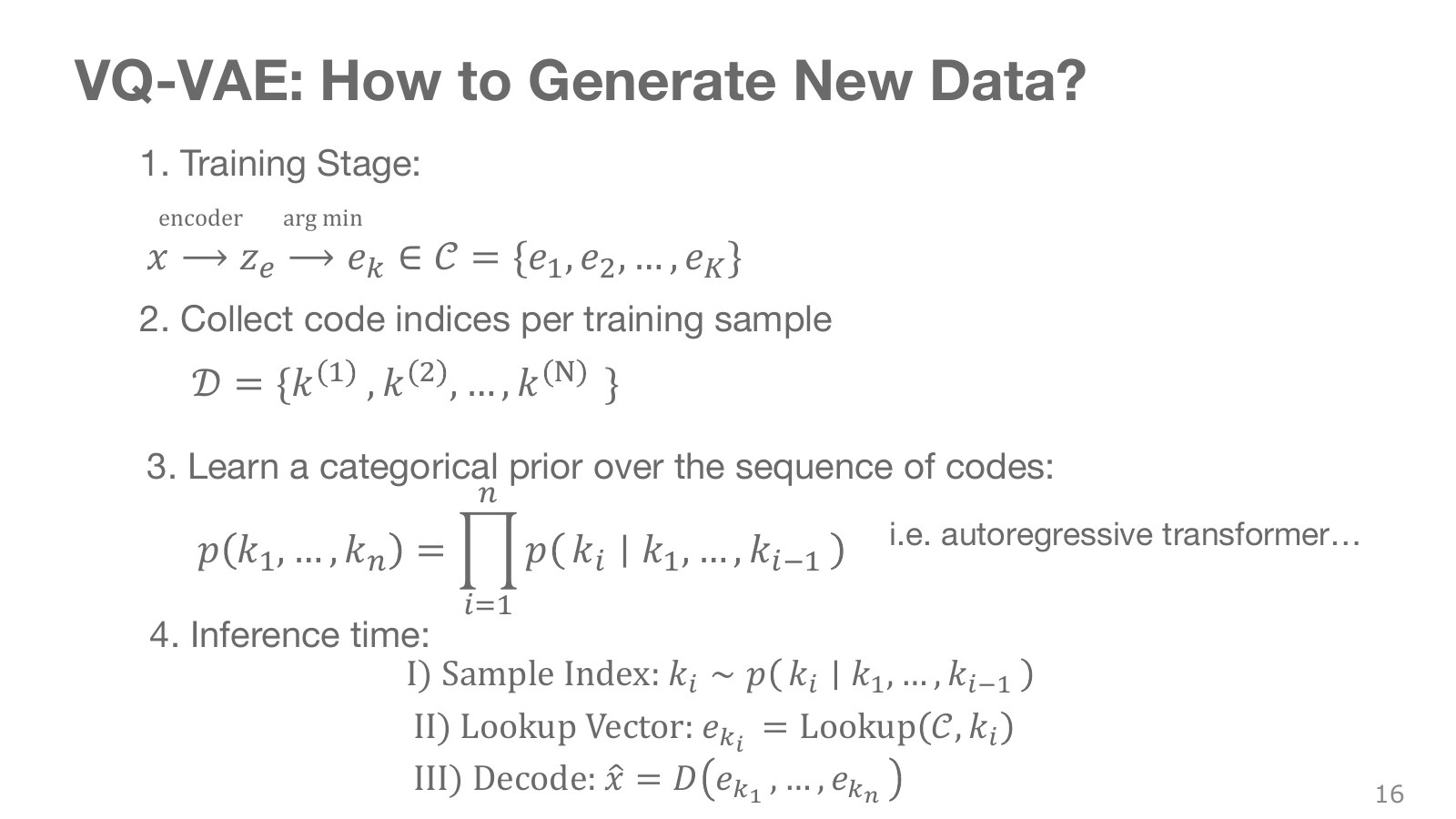
After training the encoder, codebook, and decoder in the first stage, convert data into arrays of code indices. A second-stage model can learn the distribution of these arrays. At generation time, sample indices, retrieve their corresponding vectors, and pass them to the decoder.
Explore the symbols and calculation An autoregressive distribution over code arrays
Read the equation in words
Factor a long code array's probability into next-code probabilities conditioned on preceding codes. Previously generated outputs condition later ones.
Understand each symbol
- The array of code indices to generate and its length.
- The position of the code currently being generated in the array.
- Multiply every term in the indicated range. This appears when computing the joint probability of successive choices.
- Conditional notation: the information to the right of the bar is given. This is not a division sign.
Follow the calculation
- Calculate the first code's probability.
- Condition each next code on preceding codes and multiply probabilities to the end of the array.
Check with a small example
Three conditional code probabilities 0.5, 0.8, and 0.2 give overall array probability 0.08.
An illustrative example for understanding the equation.
Predicting each next index from preceding indices preserves relationships between tokens. Sampling codes independently and uniformly at different positions can produce combinations absent from the training data. For example, if two tokens always described the same approach direction, sampling one as left and the other as right would create an inconsistent action sequence. Quantization discretizes the representation; learning its correct joint distribution remains a separate requirement.
#P018 · Discretization changes latent-space problems without removing them all
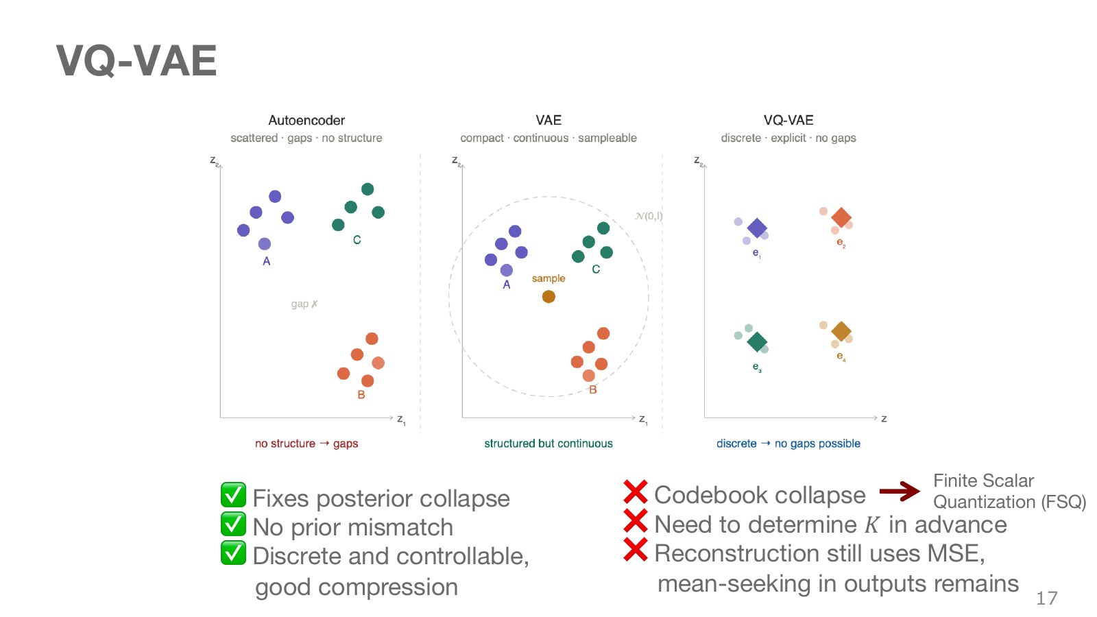
The table contrasts reconstruction-focused AEs, VAEs with continuous probabilistic latent spaces, and VQ-VAEs with discrete code lists. VQ-VAE can learn a distribution over code indices instead of fitting a prior across every point of a continuous space. Problems remain, however, including codebook collapse, where only a few codes are selected, and poorly learned code distributions. “No gaps” does not guarantee the quality of every code combination.
The FSQ paper rounds continuous values along each axis to a limited set of scalar levels, forming an implicit grid codebook. This reduces the need for a separate learned list of representative vectors and nearest-neighbor search. Networks before and after discretization, and the distribution of code use, still require learning. Representation resolution, compression, and distribution-learning difficulty must still be evaluated together.
#P019 · Distinguishing visual tokens, latent actions, and real action tokens
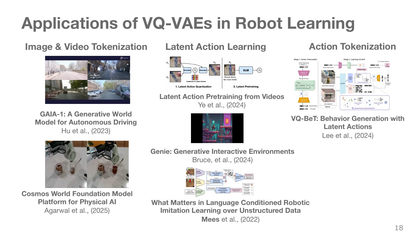
The three columns show different uses of discrete representations. First, tokenizing images or videos supports world models generating future scenes. Second, compressing changes between consecutive images into latent actions can teach patterns of change from videos without action labels. Third, tokenizing actual joint commands or action sequences represents robot-control outputs as discrete sequences.
A latent action in the middle column encodes visual change; it is not immediately a physical command specifying motor voltages. A learned mapping or decoder must connect it to actual robot actions. The left and right columns also have different aims: generating the visible world versus generating executable actions. Names such as GAIA-1, Cosmos, Genie, and VQ-BeT should not all be understood as copies of one VQ-VAE architecture.
#P020 · Diffusion learns how to reverse the progressive corruption of data
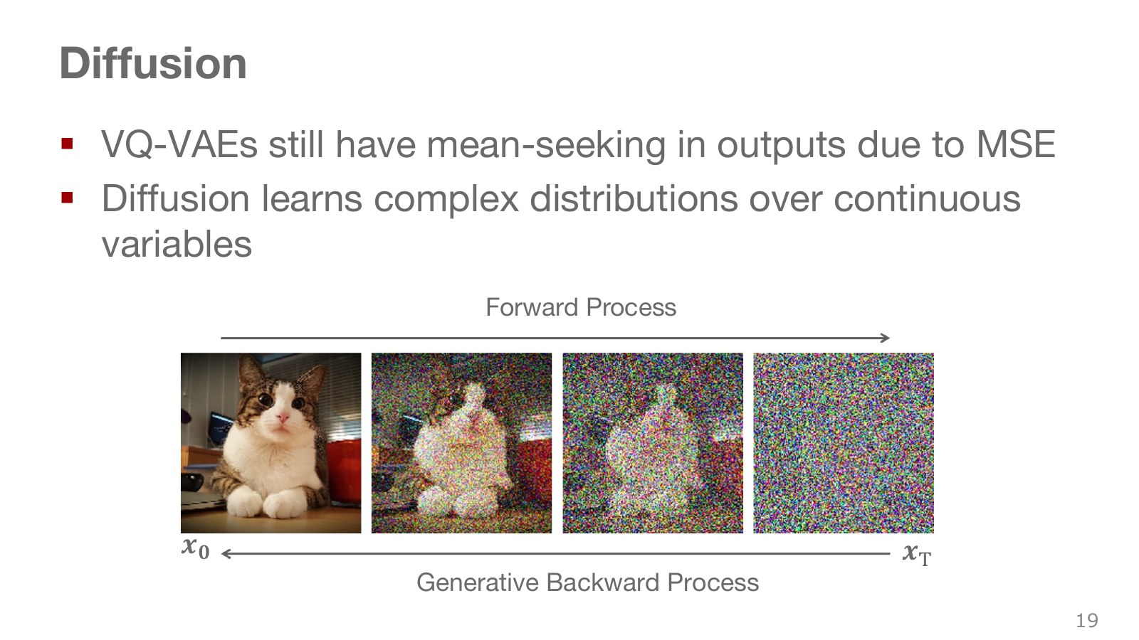
The top row, where the cat gradually becomes noise, shows how training inputs are constructed. The bottom row generates data starting from noise. During training, the original sample is known, so we can create an input at a chosen noise level and its target. During generation, the original is unknown, requiring repeated use of learned predictions.
Where latent-variable models emphasize generating outputs from a small code, diffusion constructs reconstruction problems across several noise levels. This does not mean all diffusion operates on original pixels or avoids latent spaces. Diffusion can operate on compressed latent representations too. For robot policies, the object being denoised can be an action sequence instead of an image.
#P021 · One noise-addition step combines signal attenuation with noise
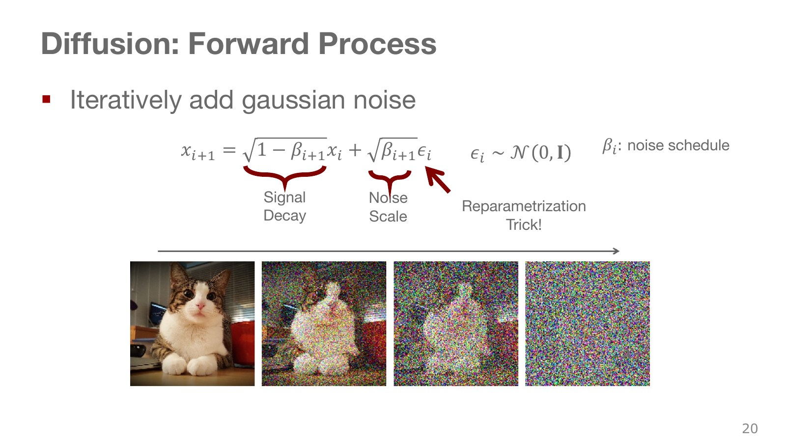
At each step, slightly shrink the current value and add independent Gaussian noise. Unlike simply accumulating noise on an unchanged signal, this also controls signal magnitude.
Explore the symbols and calculation A single forward diffusion transition
Read the equation in words
Starting with clean data, forward diffusion slightly attenuates the signal and adds Gaussian noise at each step.
Understand each symbol
- The identity matrix: diagonal entries are 1 and others 0. Multiplying a compatible vector by it leaves the vector unchanged.
- Noisy samples before and after one step. Here, indexes diffusion steps.
- The noise variance added at this step.
- A Gaussian distribution specified by its mean and covariance.
- Conditional notation: the information to the right of the bar is given. This is not a division sign.
Follow the calculation
- Scale the previous sample by the square root of the signal-retention coefficient.
- Add Gaussian noise with the specified noise variance.
Check with a small example
Noise variance 0.36 gives signal coefficient 0.8 and standard-noise multiplier 0.6. Previous value 1 with standard noise 0 gives next value 0.8.
An illustrative example for understanding the equation.
Here, is the variance of the added noise, so its square root multiplies the actual noise sample. Repeated small values gradually weaken the original features. The list specifying noise amounts at each step is the noise schedule.
The step index here is not physical robot time. Generating one action sequence at a control instant may require dozens of internal denoising calculations. Do not confuse the horizon of future robot actions with the number of neural-network denoising calls.
#P022 · The reverse process estimates the unknown original while moving backward
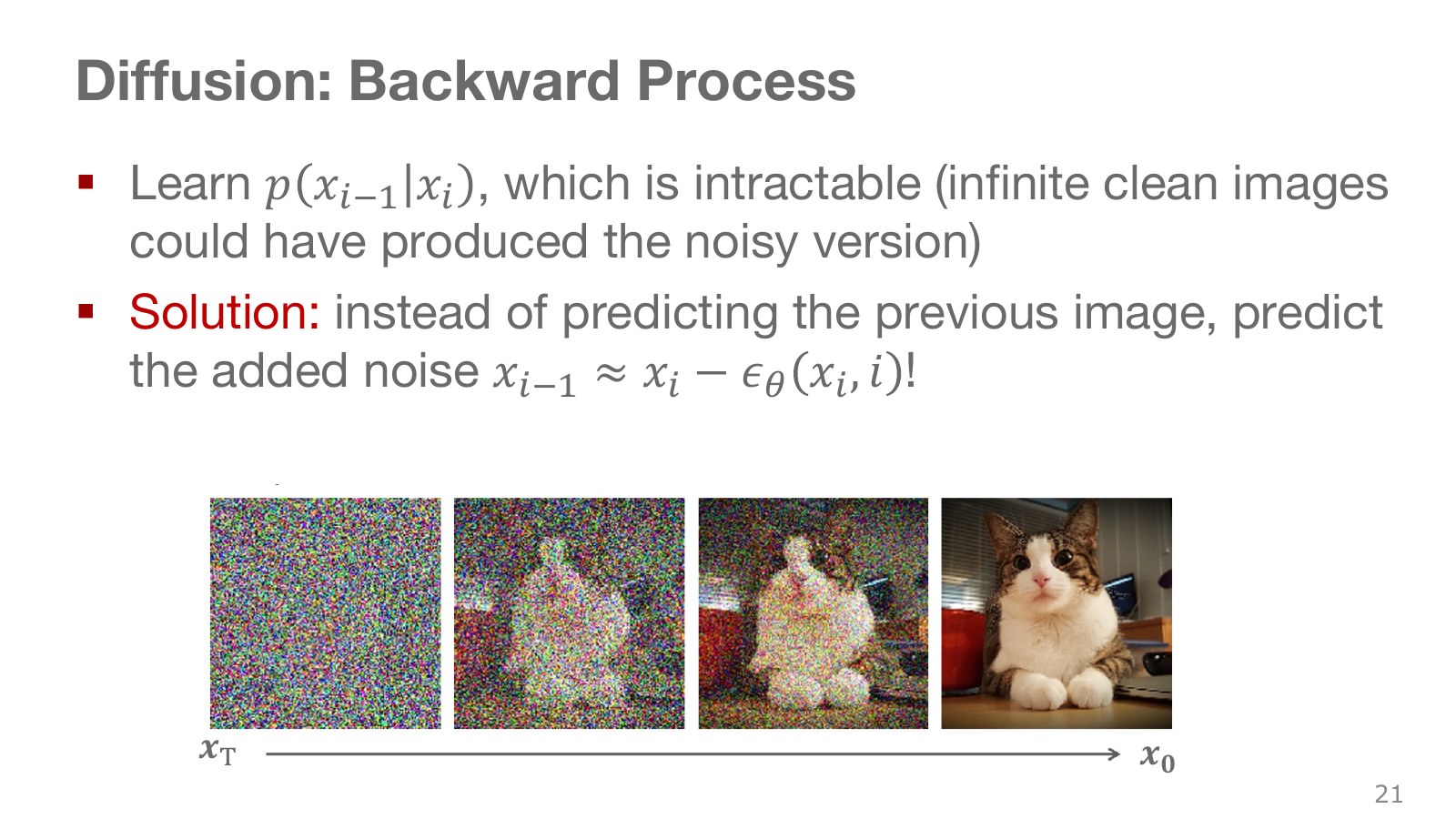
Training provides the original and the noise added to it, but execution provides only a noisy input. The model therefore estimates what to remove from the current input and noise level. Multiple originals can generally correspond to one noisy input, making denoising uncertain as well.
A common training parameterization predicts the accumulated noise from the original to the current level, rather than just the noise added in the last step. Nor does subtracting a prediction once from the current input define every diffusion sampler. Actual updates include signal and noise coefficients and next-step variance.
Conditioned on the known original, the reverse posterior can be expressed as a tractable Gaussian. At execution, however, the original is unknown, so a neural reverse process is trained to approximate it. Knowing the forward noising rule alone therefore does not solve generation.
#P023 · DDPM learns to predict noise at different noise levels
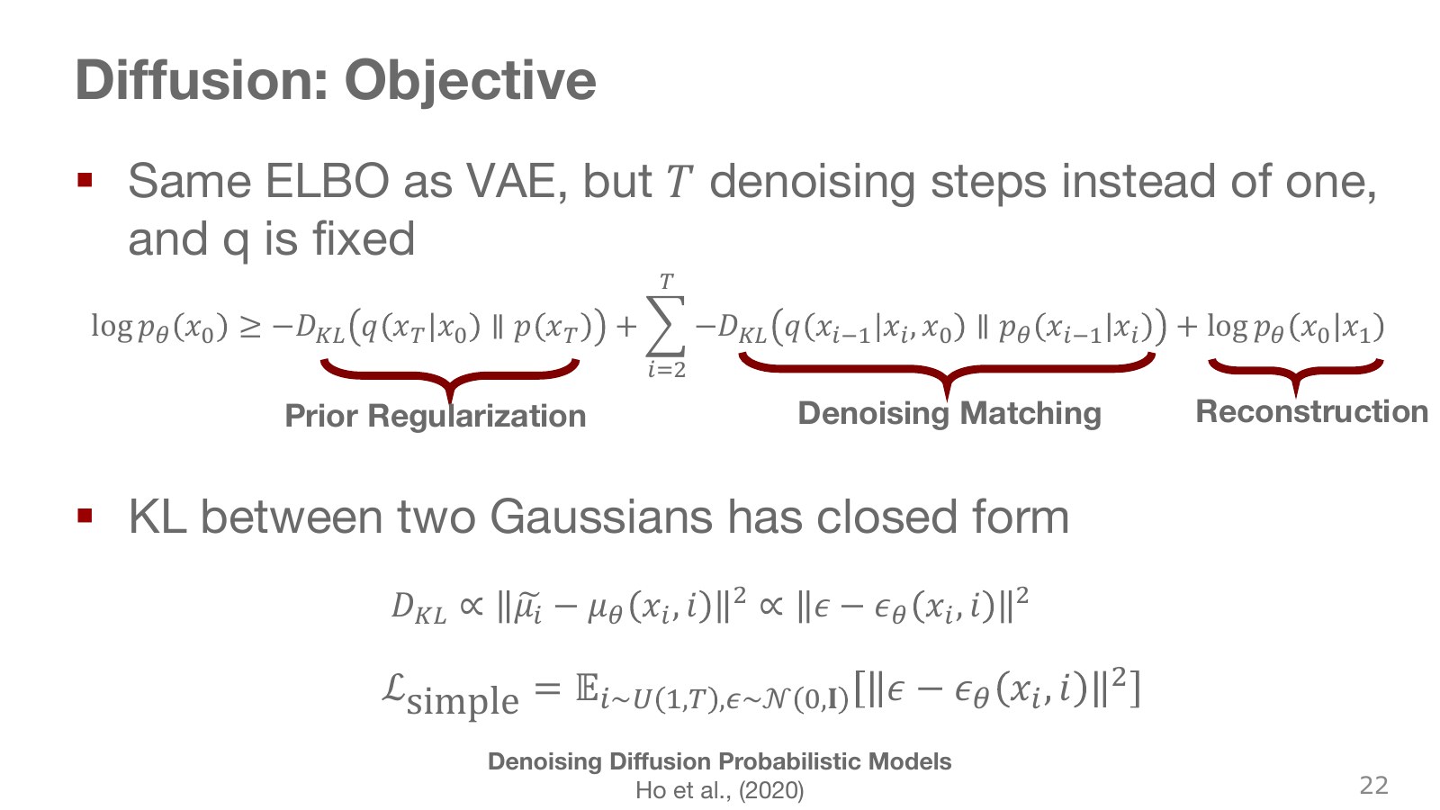
The upper equation uses a log-likelihood lower bound as in a VAE, but with multiple intermediate noisy states. The first KL aligns the final noisy distribution with the starting prior. The middle terms fit individual reverse-step distributions, and the final reconstruction term explains clean data. A rigorous bound includes expectations over the corresponding intermediate states.
A widely used simplified training objective selects a random noise level and reduces squared error between predicted and actual noise.
Explore the symbols and calculation DDPM's simplified noise-prediction loss
Read the equation in words
Train the network to predict the noise actually used in corruption. The objective learns through noise prediction rather than directly outputting the clean original.
Understand each symbol
- Sample a Gaussian noise vector with component means 0 and variances 1.
- The parameters collecting the trainable weights of the network or policy.
- The clean sample, noisy sample, and selected diffusion step.
- Noise predicted by the model from the sample and step.
- An expectation: an average over possible outcomes weighted by their probabilities.
- The squared length obtained by squaring and summing all vector components. It combines coordinate-wise errors into one nonnegative quantity.
Follow the calculation
- Add noise at the chosen level to a clean sample to construct the input.
- Average componentwise squared differences between predicted and actual noise.
Check with a small example
Actual noise [1,−1] and prediction [0.8,−0.5] give summed squared difference .
An illustrative example for understanding the equation.
Deriving the original variational objective can produce step-dependent weights. The simplified loss above should not be called term-for-term identical to the original likelihood objective. Notice that this model also uses MSE. The earlier averaging problem did not prohibit MSE itself; it concerned predicting an entire action directly as a mean. Repeatedly applying noise-level-dependent predictions during generation can produce multimodal distributions. Original DDPM paper.
#P024 · Constructing a training sample at any noise level in one step
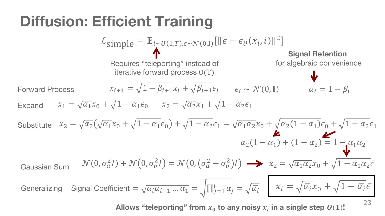
Repeated substitution of the one-step noising equation expresses the original-signal coefficient as a product of per-step signal coefficients. Independent Gaussian noises can be combined into one Gaussian by adding their variances.
Explore the symbols and calculation Definition of the cumulative signal coefficient
Read the equation in words
Multiplying per-step signal-retention ratios shows how much original signal remains. Distinguish individual step coefficients from their cumulative product.
Understand each symbol
- The per-step noise variance and signal-retention ratio.
- The cumulative product of retention ratios through the current step. The bar does not indicate an average.
- Multiply every term in the indicated range. This appears when computing the joint probability of successive choices.
Follow the calculation
- Subtract noise variance from 1 to obtain each step's retention ratio.
- Multiply retention ratios from the first step through the current one.
Check with a small example
Noise variances 0.1 and 0.2 give retention ratios 0.9 and 0.8 and cumulative ratio 0.72.
An illustrative example for understanding the equation.
Explore the symbols and calculation Direct sampling at a chosen noise level
Read the equation in words
Construct a sample at the desired noise level directly instead of executing every preceding step. Use cumulative signal and noise coefficients.
Understand each symbol
- Sample a Gaussian noise vector with component means 0 and variances 1.
- The original and a sample at noise step .
- The cumulative coefficient determining how much original signal remains.
Follow the calculation
- Prepare clean data and one standard-noise sample.
- Multiply them by square roots of the cumulative ratio and its complement, then add.
Check with a small example
Cumulative ratio 0.64 gives coefficients 0.8 and 0.6. Original 2 and noise −1 give current sample 1.
An illustrative example for understanding the equation.
This equation avoids computing the first 799 steps merely to construct one training sample at step 800. Precomputed cumulative coefficients allow direct access to the chosen level. The computational advantage concerns noise-step count; it does not eliminate data dimensionality or network computation.
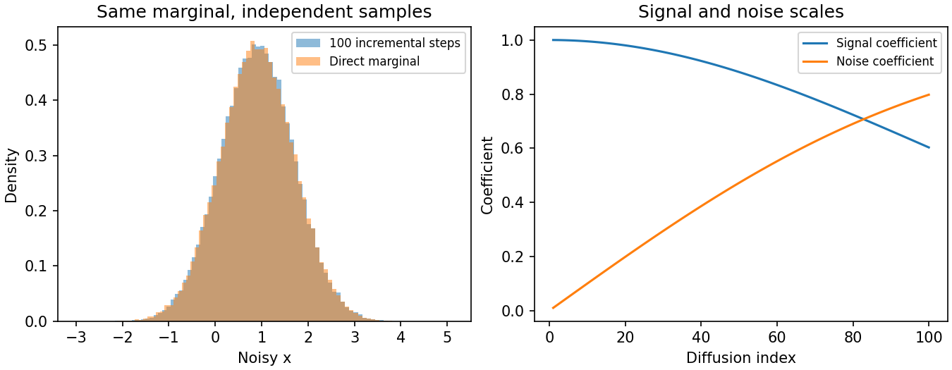
Direct and sequential samples have matching marginal distributions at each level. Independently drawn sample values need not be identical. Sampling noise independently for several times also does not reproduce the joint path of the original Markov chain.
#P025 · DDPM sampling combines a predicted mean with per-step randomness
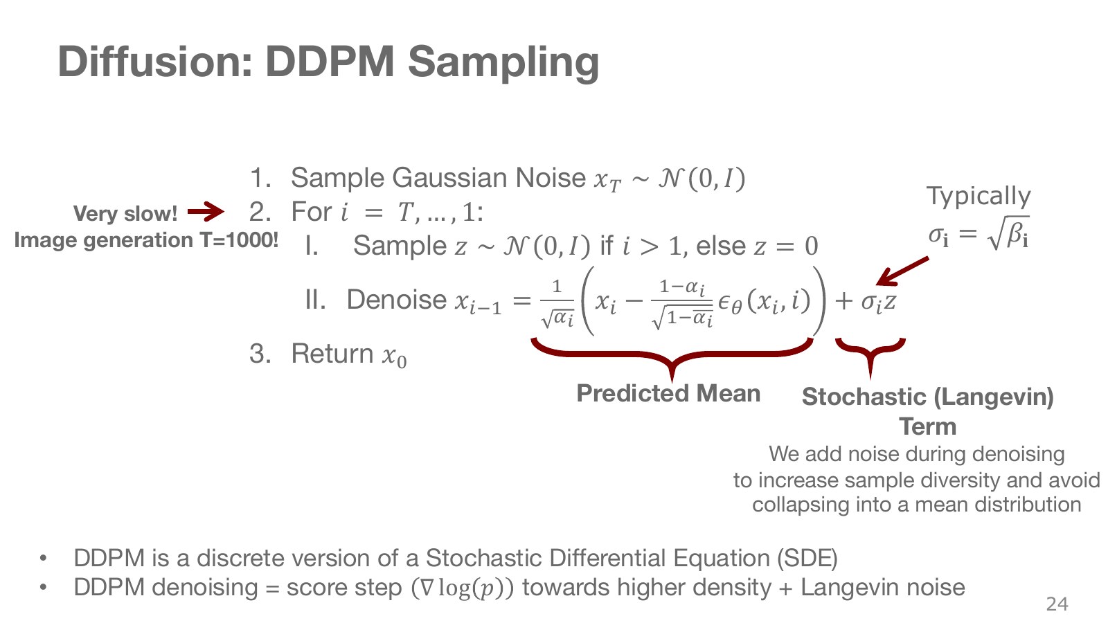
Generation begins with Gaussian noise and proceeds backward from high noise levels. Move toward a predicted mean and add noise matching the chosen reverse-process variance.
Unlike DDPM’s per-step noise addition, deterministic DDIM can follow a fixed path once the initial noise is selected. Different initial noise can still yield different outputs, so omitting per-step noise does not imply collapse to one result.
Explore the symbols and calculation The DDPM reverse sampling update
Read the equation in words
Remove part of the predicted noise from the current sample, then add fresh noise matching the chosen reverse variance to reconstruct one step.
Understand each symbol
- The parameters collecting the trainable weights of the network or policy.
- The current sample and its one-step reconstruction.
- The per-step retention coefficient, cumulative retention coefficient, and per-step noise variance.
- Predicted noise, reverse standard deviation, and newly sampled standard noise.
Follow the calculation
- Calculate the reconstruction mean using step coefficients and predicted noise.
- Add fresh noise scaled by the reverse standard deviation. The final step uses a setting without fresh noise.
Check with a small example
With predicted and fresh noise both zero and retention ratio 0.81, the mean update changes current value 0.9 to .
An illustrative example for understanding the equation.
Fresh noise is sampled from a standard normal and set to zero at the final step. Here, is the reverse-process standard deviation; it may use the square root of or another variance choice from the original paper. Using the predicted mean alone differs from sampling around it.
Do not generalize that diverse outputs require fresh noise at every step. A deterministic transformation can produce different outputs from different initial noise, as DDIM illustrates next. Nor is deleting the noise term from this DDPM equation equivalent to every deterministic sampler. Each sampler has an update matching the reverse process it approximates. Here, score means the spatial gradient of data log density, not a reinforcement-learning reward score.
#P026 · DDIM estimates a clean sample and moves to a lower noise level
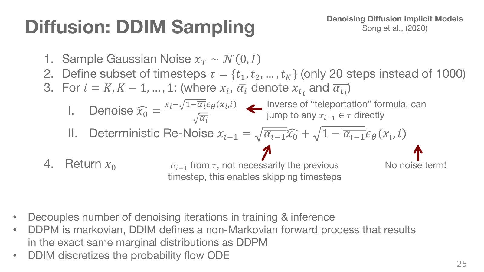
First estimate the clean original from the current input. Then combine that estimate with the predicted noise direction to construct an input at a lower noise level. Skipping intermediate steps separates the training schedule’s length from the number of predictions during execution.
Explore the symbols and calculation Estimating the original from the current sample
Read the equation in words
Rearrange the equation mixing original signal and noise to solve for the original. More accurate noise predictions yield more accurate original estimates.
Understand each symbol
- The clean original estimated at the current step.
- The current sample, cumulative retention coefficient, and predicted noise.
Follow the calculation
- Subtract the predicted accumulated-noise component from the current sample.
- Divide the remainder by the original-signal coefficient.
Check with a small example
Current sample 1.1, cumulative coefficient 0.64, and predicted noise 0.5 give .
An illustrative example for understanding the equation.
Explore the symbols and calculation A DDIM update without fresh noise
Read the equation in words
Remix the estimated original and the same predicted noise using coefficients for a cleaner step. This DDIM update adds no fresh noise.
Understand each symbol
- The current and destination diffusion steps, with smaller.
- The destination step's cumulative signal-retention ratio.
- The original estimated at the current step.
Follow the calculation
- Estimate the original and noise from the current sample.
- Recombine them using cumulative coefficients for a cleaner step.
Check with a small example
Original estimate 1, predicted noise 0.5, and new cumulative coefficient 0.81 give new sample .
An illustrative example for understanding the equation.
The expression above is deterministic DDIM with set to zero. The same conditions and initial noise produce the same output. Changing the initial noise can produce a different output, so multimodality is not lost. Fewer steps are faster, but change the effects of prediction and discretization error. Reducing 1,000 steps to 20 does not guarantee unchanged quality on every task.
Berkeley’s diffusion lecture from 52:11 distinguishes the training objective from the execution sampler. Sharing DDPM’s forward marginal distributions does not imply identical generated distributions and sample paths under every finite-step procedure. Original DDIM paper.
#P027 · Conditional generation models the distribution of outcomes needed now
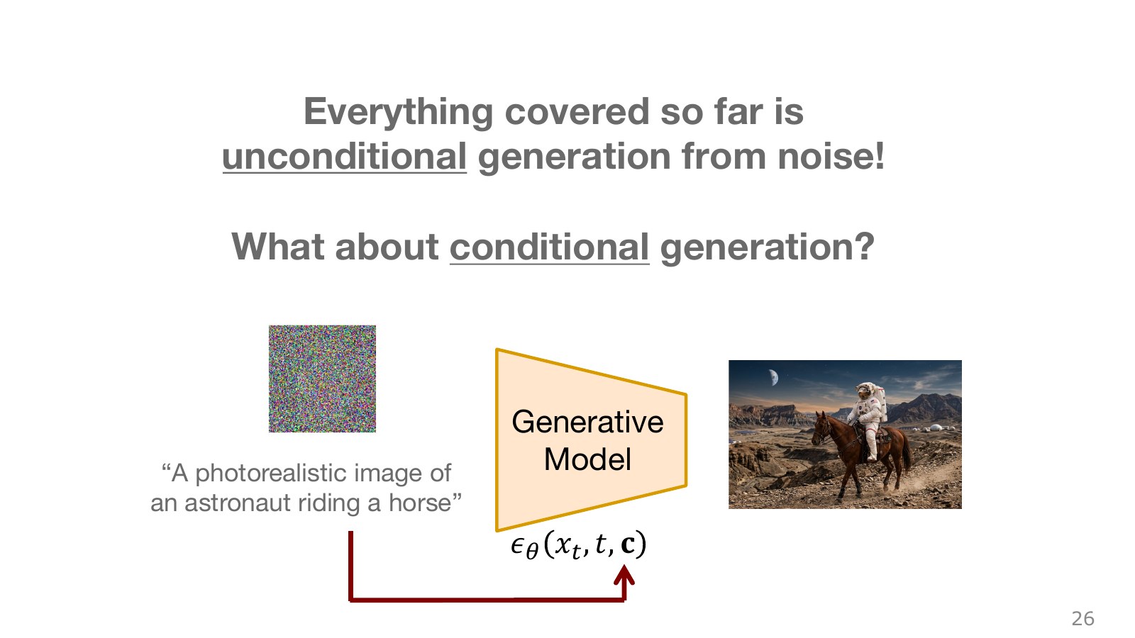
In the astronaut illustration, a text instruction constrains the image to generate. Robots can condition on camera images, proprioception—their own joint-state sensing—and language instructions. Even for the same cup, “grasp it” and “push it aside” require different action distributions.
Adding conditions to the noise-prediction network teaches observation-dependent reconstruction. The condition is not the target action itself and has a different role from a reinforcement-learning reward received afterward. Earlier diffusion equations omit conditioning only to introduce the noise process first. The latent-variable policies introduced earlier could already be conditioned on observations too.
#P028 · CFG uses the difference between conditional and unconditional predictions
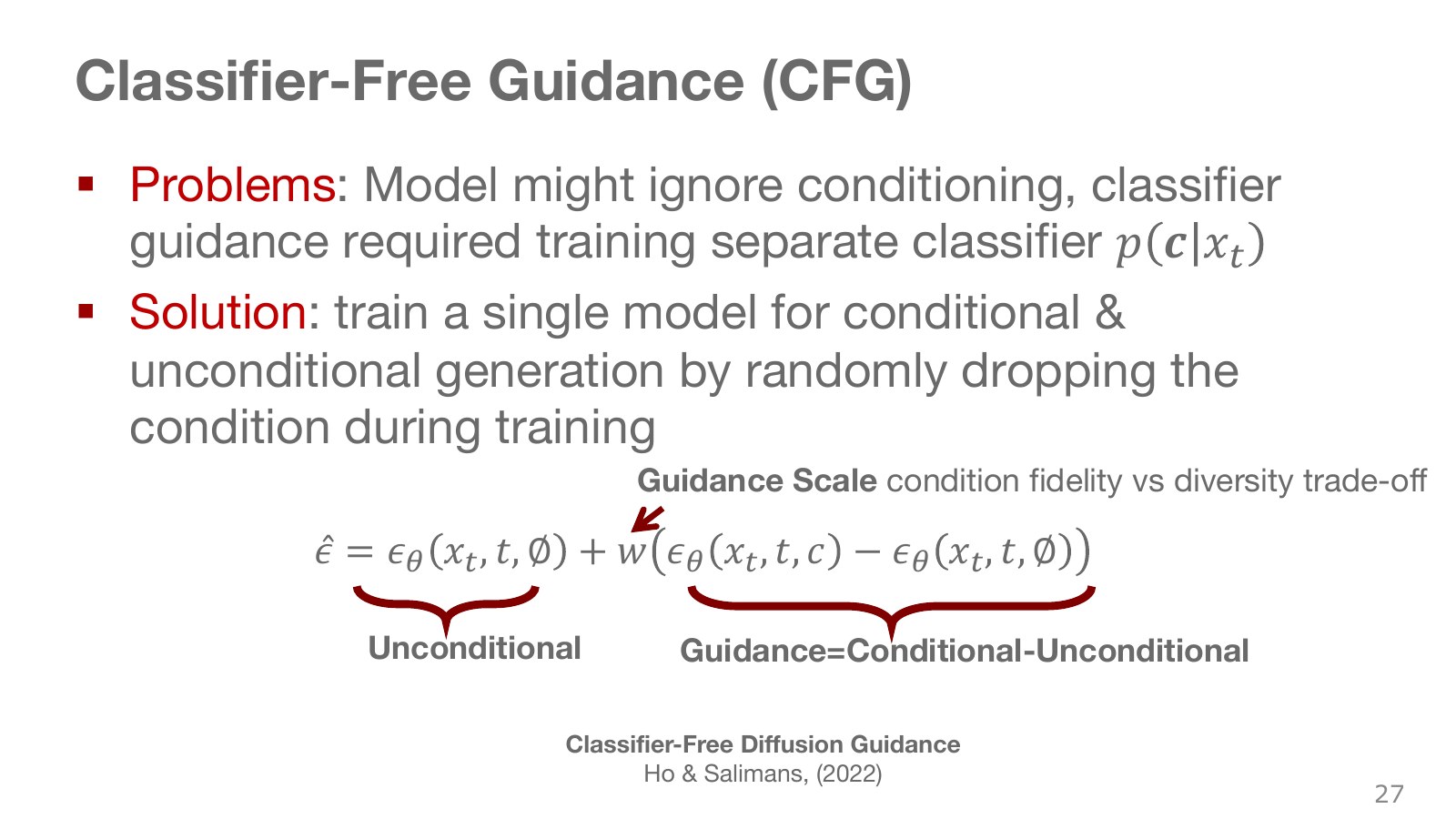
During training, replace some conditions with an empty token so the same model learns both conditional and unconditional predictions. At execution, scale the difference between those predictions to the desired strength.
Explore the symbols and calculation Combining predictions with classifier-free guidance
Read the equation in words
Start from an unconditional noise prediction and scale the change induced by conditioning. Stronger conditioning does not guarantee better results.
Understand each symbol
- Respectively, predictions with an empty condition and with conditioning. Subscripts identify these two prediction types.
- The guidance weight amplifying the conditioning effect.
Follow the calculation
- Calculate the difference between conditional and unconditional predictions.
- Scale that difference and add it to the unconditional prediction.
Check with a small example
Unconditional prediction 0.2, conditional prediction 0.5, and weight 2 give 0.8. Weight 0 gives the unconditional prediction; 1 gives the original conditional prediction.
An illustrative example for understanding the equation.
Here, is the noise prediction with an empty condition and the prediction with conditioning. The subscripts and distinguish the two predictions. Under this convention, equal to 0 gives the unconditional prediction, 1 gives the original conditional prediction, and values above 1 extrapolate farther along their difference. This can emphasize the desired condition while reducing diversity or introducing distortions.
Unlike classifier guidance, which trains a separate classifier, CFG handles both cases within one prediction model through condition dropout. “Classifier-free” does not mean generating without conditioning. Nor does every Diffusion Policy necessarily use CFG. Robot applications must choose which conditions to drop; indiscriminately removing necessary state information does not make actions safe. CFG paper.
#P029 · Diffusion Policy generates future action sequences instead of pixels
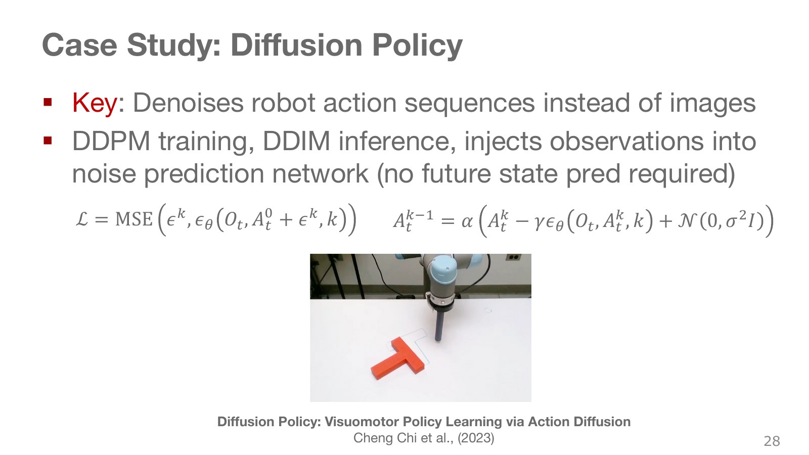
Consider pushing a -shaped object on a table to match a target outline. Bringing the object center close is insufficient; orientation and contact location also matter. Several contact sequences can lead toward the same goal, making it useful to represent multimodality in demonstrations.
Diffusion Policy adds noise to demonstrated action sequences and learns to predict that noise conditioned on the current observation. An action sequence concatenates commands for several future control instants. This basic training is imitation learning from demonstrations; it does not automatically perform reward-maximizing reinforcement learning.
Explore the symbols and calculation Noise prediction for an observation-conditioned action sequence
Read the equation in words
Add noise to a sequence of actions across multiple times, rather than one action, and predict it using the current observation.
Understand each symbol
- The sensor observation at step . It is not assumed to equal the full physical state.
- Sample a Gaussian noise vector with component means 0 and variances 1.
- The parameters collecting the trainable weights of the network or policy.
- The clean and noisy action sequences.
- The diffusion step and cumulative signal coefficient.
- The noise-prediction model that also uses observations.
Follow the calculation
- Add noise at the chosen step to the clean action sequence.
- Provide the noisy sequence, step, and observation together to predict conditional noise.
Check with a small example
Three future joint commands can form one sequence. During execution, run part of the generated sequence and replan from a fresh observation.
An illustrative example for understanding the equation.
The slide’s “add noise to actions” abbreviates the coefficient-weighted process above. Outputs are future actions, not necessarily predictions of future images or world states. A receding-horizon approach can predict a long action sequence, execute only part of it, then replan from a fresh observation. Diffusion Policy paper, videos, and code.
#P030 · Share observations within one planning cycle while repeatedly updating the action array
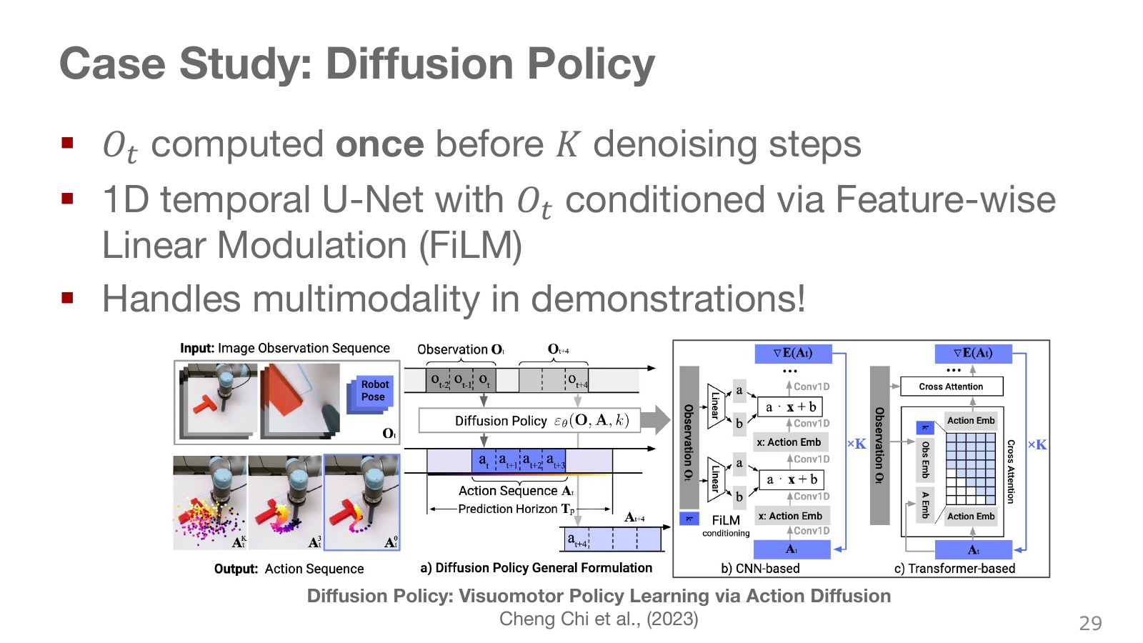
The images on the left show camera observations and joint states conditioning the transformation of noise into a coherent action sequence. The middle timeline separates prediction and execution horizons. Observing again after execution allows responses to environmental changes.
Camera and robot-state encoding is paid once per planning cycle, and the representation is shared across denoising steps. In the temporal U-Net variant, FiLM adjusts internal feature scales and shifts using the observation; the Transformer variant attends to observations. Diffusion Policy project
The U-Net’s 1D axis on the right is the action sequence’s time axis. Downsampling gathers broader context, then upsampling reconstructs actions at each time, with skip connections preserving detail. FiLM derives feature-specific scales and shifts from conditioning to modulate intermediate activations. In a Transformer variant, action tokens can attend to observation tokens.
Computing observation features once means reusing them across denoising steps within one action-sequence generation cycle. It does not mean reading the camera only once during the entire robot run. Normalizing action units and ranges also matters. Treating translations in meters and rotations in radians as if they shared a numerical scale changes the balance of learning.
#P031 · Extending a task-specialized policy to multiple tasks
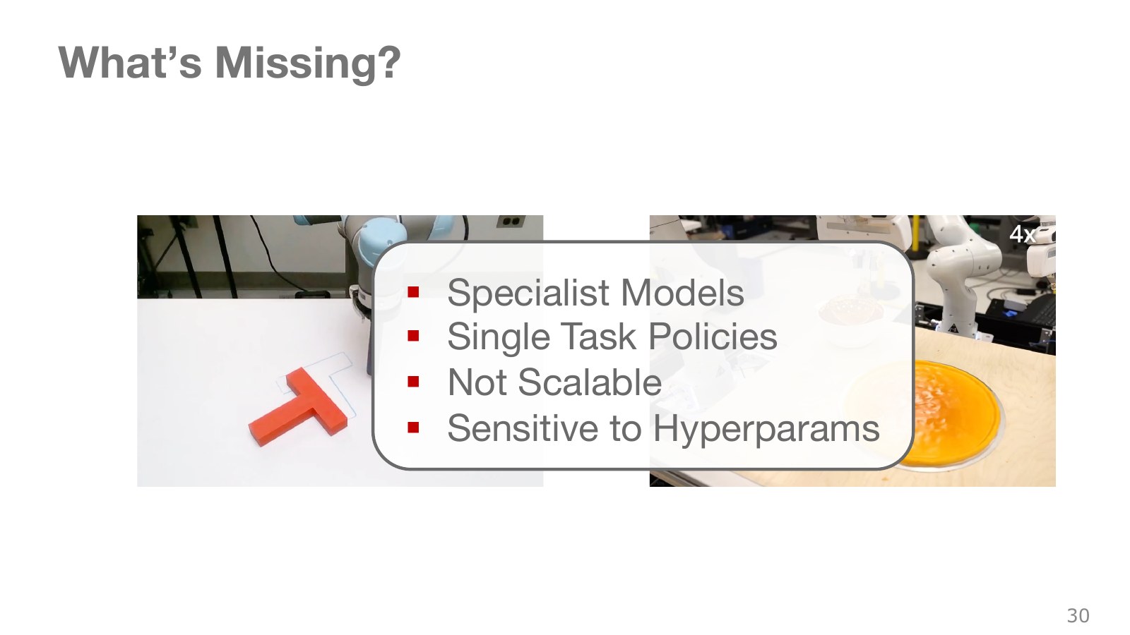
Different objects, tools, and contact modes in the photographs call for different action distributions. A specialist trained for one task does not readily transfer unchanged to another task or robot. Beyond dataset size, observation formats, task conditions, action dimensions, and units must be handled together.
The original lecture discusses training sensitivity and scaling difficulties in the early Transformer version of Diffusion Policy. This does not mean diffusion policies are fundamentally unable to learn multiple tasks. Octo and DiT Policy, discussed next, extend in that direction through changes to data and architecture. Successful single-task demonstrations and generalization under varied conditions require separate evaluation.
#P032 · Octo connects multiple robot datasets through shared representations and an action-generation head
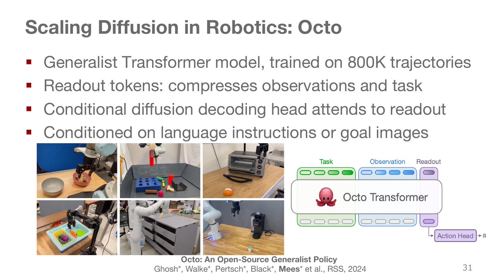
The architecture below separates language or goal images, observation tokens, readout tokens, and an action head. A token is one information slot processed by the model. Readout tokens gather task and observation information into a representation for action output. A small diffusion head then generates an action sequence conditioned on that representation.
The Octo paper studies a general robot policy trained on approximately 800,000 trajectories from Open X-Embodiment. Each trajectory contains multiple control steps, so this is not 800,000 individual actions. Its diffusion action head is a small MLP. Do not conflate the readout’s attention-based information aggregation with the action head receiving that result, as if both were the same cross-attention block.
The point is that pretrained representations can be adapted to new robots, not that a download instantly matches every robot’s joint ordering and units. Input/output adapters and additional training conditions are required.
#P033 · DiT Policy injects conditions through normalization-layer scales and shifts
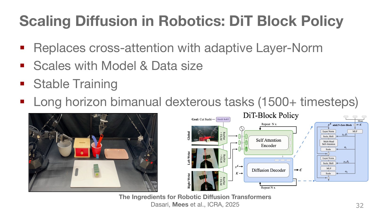
The observation encoder combines images and robot states, while the action generator updates noisy action tokens. AdaLN means adaptive layer normalization. It conveys observations and noise levels by conditioning how normalized features are scaled and shifted. This connects to FiLM’s idea of modulating internal features with conditions.
The DiT Policy paper reports stability and complex manipulation performance under particular architectural changes and training choices. This is not proof that cross-attention is unnecessary in every Transformer. A long task such as sushi cutting may span 1,500 control steps, which is different from the number of diffusion steps generating one action sequence. One measures control time in the environment; the other measures internal generation computation.
#P034 · Flow matching learns a velocity field from noise to data
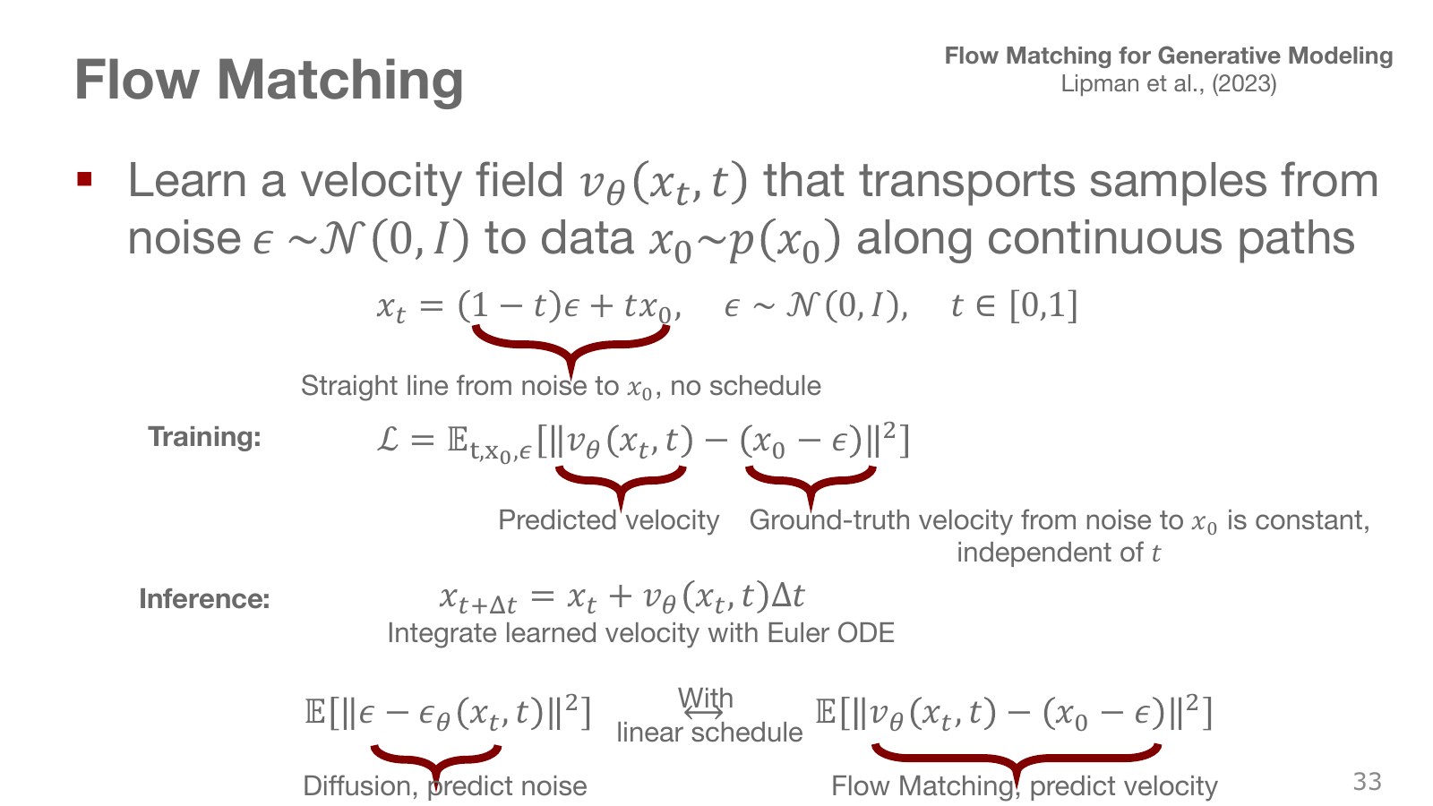
Sample one noise value and one data example, then connect them with a straight line. Mixing them so that time 0 is noise and time 1 is data produces training examples anywhere along the path.
Explore the symbols and calculation A straight probability path and the paired samples' target velocity
Read the equation in words
Construct a straight path connecting noise and actual data and define its target velocity. Generation time 0 denotes noise and 1 denotes data.
Understand each symbol
- Sample a Gaussian noise vector with component means 0 and variances 1.
- Generation time running from 0 to 1, distinct from robot execution time or a trajectory label.
- The actual data and intermediate path sample.
- The target velocity along the path joining a sample pair, not an RNN memory vector or control torque.
Follow the calculation
- Choose endpoints and linearly mix them according to time.
- Differentiating with respect to time makes target velocity the endpoint difference.
Check with a small example
Noise −1 and data 3 give intermediate value 1 at time 0.5 and target velocity 4.
An illustrative example for understanding the equation.
Explore the symbols and calculation The flow-matching velocity-regression objective
Read the equation in words
Train the model to predict target path velocity from an intermediate sample and generation time. Regression reduces squared differences between target and predicted vectors.
Understand each symbol
- The parameters collecting the trainable weights of the network or policy.
- The predicted velocity vector field over intermediate position and generation time.
- The target velocity formed from data minus noise in the preceding equation.
- The flow-matching loss: mean velocity-prediction error.
- An expectation: an average over possible outcomes weighted by their probabilities.
- The squared length obtained by squaring and summing all vector components. It combines coordinate-wise errors into one nonnegative quantity.
Follow the calculation
- Sample a noise–data pair and intermediate generation time to construct a path sample.
- Compare predicted velocity against that pair's target velocity.
Check with a small example
Target velocity 4 and prediction 3 give one-dimensional squared loss 1. Where different paths overlap, the optimal regressor at a location is conditional mean velocity.
An illustrative example for understanding the equation.
A vector field specifies which direction and how far to move given the current position and generation time. Generation starts from fresh noise and integrates this field. The simplest Euler method adds current velocity multiplied by a small time interval to the position.
Explore the symbols and calculation One Euler integration step
Read the equation in words
Move for a short time using the velocity predicted at the current location. This is the simplest numerical integration of a learned field from noise to data.
Understand each symbol
- The parameters collecting the trainable weights of the network or policy.
- The sample at the current generation time.
- The time interval for one integration step.
- The model's predicted velocity along the generation path.
Follow the calculation
- Predict velocity from the current generation time and sample.
- Multiply velocity by a small time interval and add it to the current sample.
Check with a small example
Current value −1, predicted velocity 4, and time interval 0.1 give new value −0.6. Repeated large steps can increase integration error.
An illustrative example for understanding the equation.
A particular noise–data pair has constant target velocity, but the overall learned velocity field is not constant everywhere. When several pairs pass near the same intermediate location, the model learns their conditional mean velocity, and paths obtained by integrating the field can curve. Although this also uses MSE, its generative structure differs from directly outputting one mean action. Generation time is not physical robot-motion time: the robot does not execute every intermediate action array along the generation path.
Straight interpolation is the path selected in this lecture; flow matching as a whole need not use only this path. Original Flow Matching paper.
#P035 · Rectified flow retrains on generated pairs to straighten paths
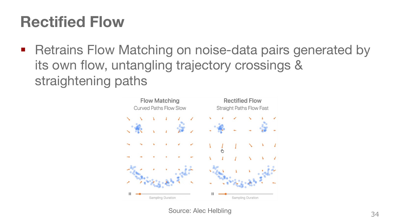
Randomly pairing arbitrary noise and data can produce crossing straight lines. When different target directions overlap at an intermediate location, representing them with one smooth vector field can lead to curved flow. The difference between the left and right curves illustrates an attempt to simplify this transport.
First train a flow, then follow it from fresh noise to an endpoint. Pair that initial noise with the reached endpoint and train again. This recoupling and retraining is called reflow. It uses pairs connected by the current model instead of the original independently sampled pairs.
Straighter paths can be easier to approximate with fewer integration steps. This does not make every flow exactly straight or guarantee equal quality in one step. Learning error, integration error, and representational limits remain. Also distinguish crossings of straight training pairs from crossings at the same space–time point by actual solution paths of a smooth ODE satisfying uniqueness conditions. Rectified Flow paper.
#P036 · π₀ generates continuous action sequences conditioned on visual and language representations
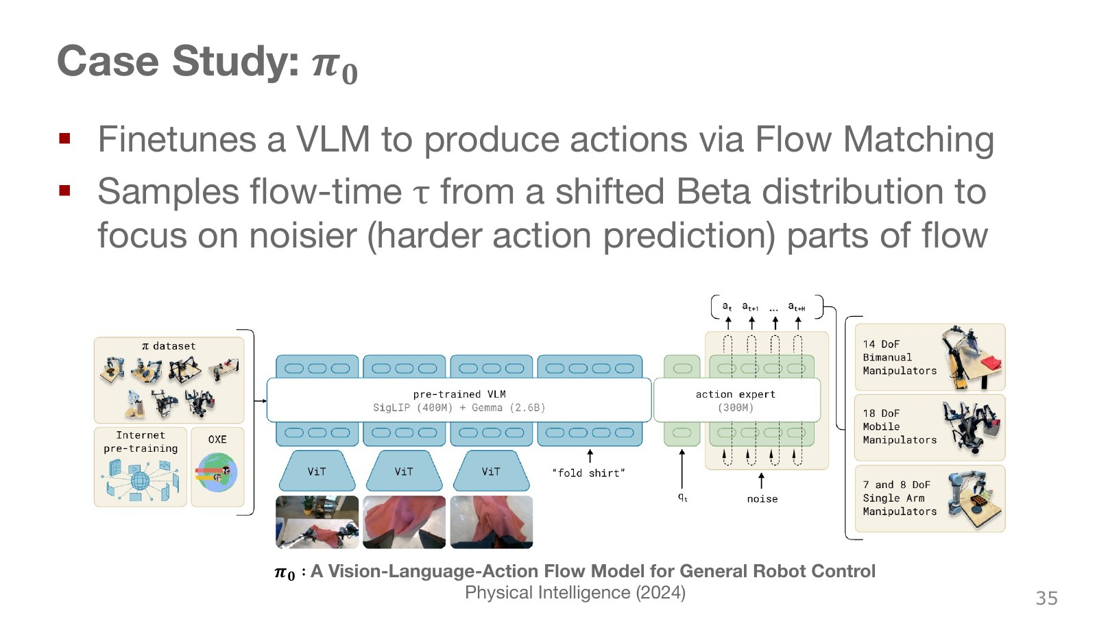
The left side shows robot data and Internet pretraining data; the middle contains a vision–language model; the right contains an action expert. It uses representations interpreting camera images and instructions such as “fold the shirt,” while robot-specific weights process joint states and noisy actions. The dual-arm, mobile, and single-arm robots illustrate its intended range of embodiments.
Rather than sampling every flow time equally often, the π₀ introduced in the lecture gives greater weight to high-noise regions. Which noise levels are practiced frequently during training and how many integration steps are used at execution are separate choices. π₀ paper
In Section 4 and Appendix B of the original π₀ paper, generation time runs from 0 for noise to 1 for clean actions, matching this chapter’s straight-flow equations. Mixing this with diffusion notation that uses zero for clean data can reverse the integration direction in code. Hold observations fixed, start from noisy actions, integrate from 0 to 1, execute part of the resulting action sequence, and observe again.
Instead of uniform training-time sampling, the model uses a shifted Beta distribution emphasizing smaller times with more noise. The appendix specifies an upper bound of 0.999 and a transformed Beta(1.5,1). This allocates training effort to regions where predicting actions from observations is difficult; it is not a mandatory rule for every flow model.
Model sizes and module names in the figure describe the original configuration cited by this lecture. Vision–language pretraining does not mean Internet images carry actual motor-command labels. Robot action data and flow training provide that connection. Joint training across robots also requires aligning action dimensions, normalization, and input/output mappings.
#P037 · Comparing distribution representations and execution procedures together
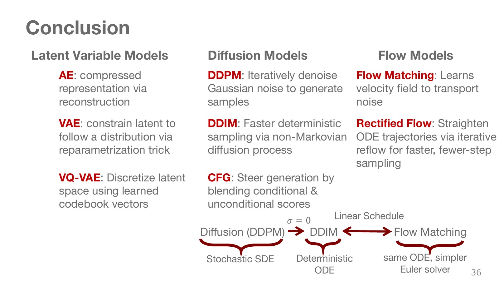
Rather than asking which family is newest, first ask what it predicts and how it generates samples.
| Family | Core learning target | Generation procedure | Robot-specific question |
|---|---|---|---|
| VAE | Probabilistic latent representations and a decoder explaining inputs | Sample a prior code and reconstruct | Can codes be sampled without target actions at execution? |
| VQ-VAE | Discrete codebook and reconstruction, plus a separate code distribution | Sample indices, retrieve vectors, and reconstruct | How do code combinations map to actual actions? |
| DDPM and DDIM | Predictions at multiple noise levels | Iteratively recover data from noise | Are generation steps, latency, and action horizon distinguished? |
| Flow matching | A velocity field over position and generation time | Integrate the field from noise | Are time direction and integration intervals consistent? |
Diffusion noise prediction and flow velocity prediction can be connected through transformations under selected probability paths and time parameterizations. This does not make finite-step DDPM, DDIM, and every flow sampler identical algorithms or guarantee identical quality. Consider discretization, objective weights, conditioning, and computation together.
The ability to generate diverse actions does not guarantee good actions. A dataset with many failures can teach their distribution too, and a model unaware of constraints can generate dangerous commands. Generative models provide policy representations; deciding what they learn and how they are evaluated remains a design problem for imitation learning, reinforcement learning, and control systems.
#Calculations run and checked for this article
The executable code and results are available so the equations can be explored without a robot. Calculations cover collision by averaging two detours, the ELBO and KL gap in a Gaussian latent model, reparameterization derivatives, true quantization derivatives versus STE, diffusion marginals, DDIM clean-sample reconstruction algebra, CFG weights, and flow integration error.
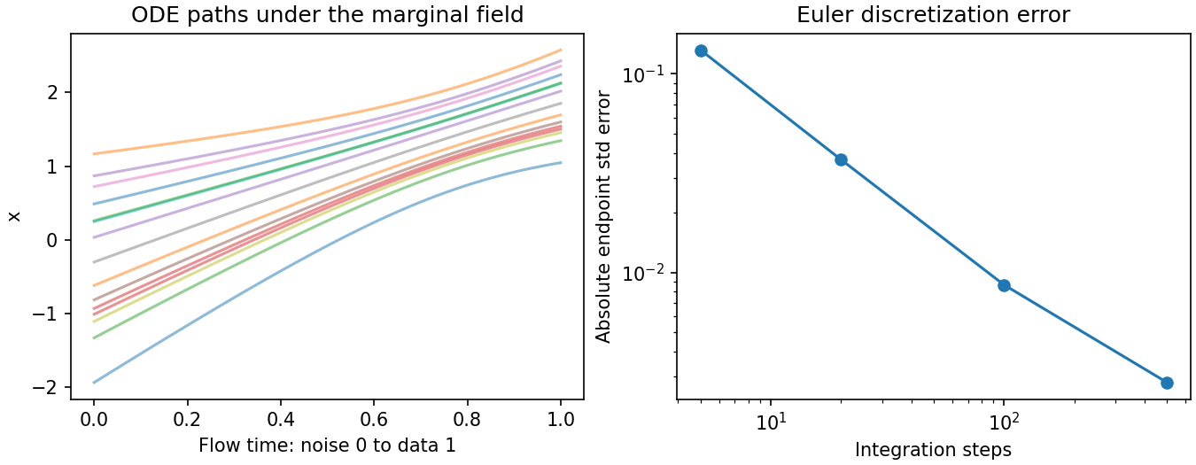
These examples are numerical calculations using known probability distributions. The DDIM check uses ground-truth noise and therefore does not evaluate a learned noise predictor. They also do not represent training VAE or Diffusion Policy networks, completing the official assignment, running robot physics simulation, or executing hardware. For executable robot examples, consult the official Diffusion Policy code and the project paper’s simulation and experimental settings.
#Related lectures and original sources
- Berkeley CS294-158, Deep Unsupervised Learning 2024: Lecture 4 on latent variables and VAEs, and Lecture 6 on diffusion. These supplement the ELBO-gap explanation and distinction between training and sampling.
- Original VAE paper · VQ-VAE: starting points for probabilistic latent representations, reparameterization, and codebook learning.
- DDPM · DDIM · CFG: read noise-prediction objectives separately from generation procedures.
- Diffusion Policy · Octo · DiT Policy: compare action sequences, conditioning, and multitask scaling.
- Flow Matching · Rectified Flow · π₀: learning velocity fields and connecting them to action generation.
- Cheng Chi’s invited talk: at 4:30–7:31, hardware, data, components, and procurement are discussed as essential system conditions alongside algorithms. This recording supplements implementation context beyond the model; it is not assumed to be an additional lecture deriving Diffusion Policy equations.
Copyright in the slides and lecture belongs to Oier Mees and the rights holders of each cited resource. This English edition translates JJo’s Korean explanation of the original materials; JJo generated the article’s numerical figures. Figures and videos from cited papers and models remain subject to their original authors’ rights. Oier Mees · ETH Computer Vision and Geometry Group.