대조 표현학습은 무엇을 같은 대상으로 묶고, 무엇을 비교 대상으로 둘지를 설계한다. 손실의 이름만 같아도 positive의 정의, 후보 수, gradient가 흐르는 경로와 평가 방식이 달라지면 다른 학습이다. 이 글은 CPC·SimCLR·MoCo·CLIP의 연산과 계산을 중심으로, BYOL·Barlow Twins·clustering·SupCon의 차이를 연결한다. 작은 행렬과 숫자는 별도의 해설 예제이고 논문 실험 결과와 구분한다.
#8.1 metric learning에서 contrastive learning으로
거리 기반 학습은 정답 class logit만 맞히는 대신 표현 사이의 관계를 제약한다. triplet은 anchor a, positive p, negative n의 상대 거리를 비교한다.
anchor와 같은 의미의 view에는 높은 similarity를, 다른 sample에는 낮은 similarity를 부여하도록 embedding space를 학습한다.
계산 예제. 제곱거리가 positive=0.2, negative=0.3이고 margin=0.5라면 hinge loss는 max(0,0.2−0.3+0.5)=0.4다. negative 거리가 1.0이면 loss=0이다. 이미 충분히 멀어진 negative에서는 이 triplet이 gradient를 주지 않는다는 뜻이다. “더 어려운 negative만 고르면 된다”도 일반 해답은 아니다. 실제 같은 의미의 다른 sample을 negative로 선택했다면 그 어려움은 좋은 감독 신호가 아닐 수 있다.
여기서 다루는 triplet 예와 이후 InfoNCE는 같은 식이 아니다. 전자는 margin 위반을, 후자는 후보 중 positive를 찾는 정규화된 점수 문제를 사용한다. 원래 논문마다 positive와 negative의 sampling 규칙을 함께 기록해야 한다.
#8.2 InfoNCE: 올바른 쌍을 고르는 분류 문제
CPC는 encoder로 입력을 표현하고, context로부터 미래 등의 관련된 latent를 구별하도록 학습한다. 원본 Figure 1에서는 입력 인코딩, context를 모으는 autoregressive 경로, 미래 표현에 점수를 주는 경로를 구분한다. CPC 원문 Figure 1 및 §2, 1807.03748v2을 기준으로 읽으며, 이 개요 그림을 이미지 두 장의 증강만 사용하는 SimCLR 도식과 같은 것으로 소개하지 않는다.
후보 집합에 positive 하나와 negative들이 있고, 점수를 s라고 쓰면 손실을 다음처럼 읽을 수 있다. 아래는 일반적인 softmax 표기로 풀어 쓴 식이다.
Positive는 분자뿐 아니라 분모에도 들어간다. 분모가 “negative들만의 합”이라고 설명하면 확률과 cross entropy의 의미가 달라진다. 모든 후보 점수가 같고 후보가 N개라면 positive 확률은 1/N, 손실은 log N이다. 후보가 네 개면 약 1.386294 nats다.
Mutual information lower bound와 연결할 때 N은 해당 유도에서 positive를 포함한 전체 후보 수다. negative를 marginal에서 뽑는 등 유도의 sampling 조건도 필요하다. 아무 hard-negative mining으로 바꾼 뒤 원래 MI bound를 그대로 적용하지 않는다. log N이 bound의 표현 범위를 제한한다는 사실은 “N을 늘리면 실제 의미 정보가 반드시 늘어난다”는 보장이 아니다. CPC의 실험은 여러 데이터 영역에서 얻은 representation의 유용성을 평가하며, 생성 이미지의 FID를 평가한 논문으로 바꾸어 소개하지 않는다. CPC, §2.3 및 실험
구현에서의 점검. exp를 먼저 전부 계산하면 큰 logit에서 overflow할 수 있으므로 log-sum-exp를 쓴다. temperature를 적용한 score인지 원래 cosine인지 구분한다. 미니배치가 작아 유효 negative가 사라지거나, 동일 데이터가 여러 rank에 중복돼 false negative가 늘어나는 경우도 별도 점검한다.
#8.3 augmentation이 곧 학습할 invariance다
같은 이미지에서 두 view를 만들면 두 view 사이에서 무엇을 지워도 “같다”고 볼지를 선택한다. 이는 단순한 데이터 수 증가가 아니다. crop·color distortion·blur가 어떤 downstream 정보를 제거할 수 있는지 생각해야 한다. SimCLR, §3
사고 예제. 하나의 영상에 고양이와 자동차가 함께 있는데 두 crop이 각각 다른 물체만 남겼다면 instance 기준 positive는 만들어졌지만 두 view의 의미가 같다는 가정은 약해진다. 반대로 색이 중요한 불량 판정 과제에서 강한 색 제거를 사용하면 필요한 단서까지 버리게 만들 수 있다. 이는 데이터와 목적에 대한 설계 추론이며, 해당 논문에서 이 특정 산업 데이터를 실험한 결과가 아니다.
따라서 증강 범위, positive 생성 규칙, 학습에 사용한 정보와 downstream 목표를 같이 적는다. 어떤 증강이 표준 benchmark에서 좋았다고 모든 센서·의료·산업 영상에 같은 설정을 무비판적으로 적용하지 않는다.
#8.4 SimCLR: 단순하지만 batch와 증강에 민감한 기준선
SimCLR은 동일 이미지의 두 증강 view를 positive로 사용하고, batch 안의 다른 view들을 비교 대상으로 삼는다. 원본 framework 그림에서 augmentation t, encoder f, projection head g를 각각 구분해야 한다. Chen 등, 2002.05709v3, §2, Figure 2
같은 이미지에서 만든 두 view를 positive pair로 두고, batch 안의 다른 view들을 negative로 사용한다.
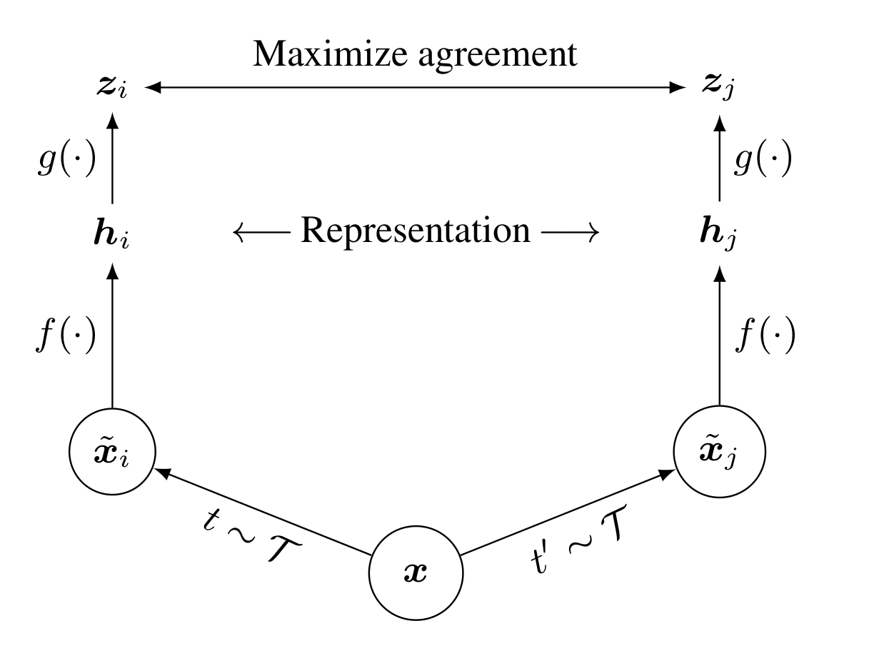
하나의 x에서 갈라지는 t와 t′는 독립적으로 뽑은 증강이다. f와 g는 서로 다른 역할이며 두 branch의 f는 가중치를 공유한다. 위쪽 z에서 학습하는 목적과 가운데 h를 downstream에 사용하는 선택을 구분한다.
Ting Chen et al. · 2002.05709v3 · 원논문 · 원문 속 그림 · 크게 보기 원논문 도판 발췌. 원문 PDF에서 도판 영역만 잘라 고해상도로 렌더링했다. 한국어 해설은 별도 작성. 원권리자의 권리가 유지되며 블로그 코드의 MIT 라이선스가 도판의 재배포 허락을 뜻하지 않는다.#N개 이미지, 2N개 view, 2N−1개 후보
위 식은 cosine similarity다. 이를 loss에 넣으면 다음 NT-Xent 형태가 된다. j(i)는 anchor i의 positive index다.
이미지 N개에서 view를 두 개씩 만들면 2N개의 embedding이 된다. anchor 자기 자신만 제외하므로 분모에는 2N−1개 후보가 남는다. 이 중 하나가 positive이며 negative는 2N−2개다. 대칭으로 두 방향 모두 학습하므로 anchor 수는 2N이다.
N=2라면 view를 [a1,a2,b1,b2]로 놓자. a1의 positive는 a2, negative는 b1·b2다. a1 자신을 제외한 분모에 a2가 들어간다. 저장 순서를 [a1,b1,a2,b2]로 바꾸면 positive index도 바뀐다. “정답 index는 언제나 옆 칸”이라는 코드는 augmentation concatenation 순서에 따라 틀릴 수 있다.
해설용 shape 예에서 ResNet-50의 pooled h는 [2N,2048], projection z는 [2N,128]이다. 정규화한 z와 zᵀ를 곱하면 [2N,2N] similarity matrix다. projection head는 학습을 위한 비교 공간을 만들고, 논문의 linear evaluation에는 h를 사용한다. SimCLR, §2, §4
#Temperature를 숫자로 확인하기
anchor에서 positive의 cosine이 1, 두 negative의 cosine이 0과 −1이라고 가정하자. τ=0.5라면 logits는 [2,0,−2]가 된다.
τ=1이면 loss는 약 0.407606이다. 이 구성에서는 temperature를 낮추면 이미 가장 높은 positive에 확률이 더 몰린다. 그러나 positive보다 높은 false negative가 있으면 그 잘못된 비교도 더 세게 강조할 수 있다. 이 계산만으로 작은 τ가 항상 좋은 representation을 만든다고 결론낼 수 없다.
점수를 temperature로 나누기 전의 similarity를 s_j라고 하면 아래 도함수가 나온다. cosine 정규화 이전 embedding까지 미분하려면 normalization의 chain rule도 추가로 필요하다.
메모리 예제. N=4096이면 8192×8192 matrix의 원소는 67108864개, float32 한 장은 256 MiB다. gradient·encoder activation·optimizer 상태를 제외한 값이다. 이것을 전체 training GPU memory라고 쓰면 안 된다. blockwise 계산 등으로 구현 비용을 바꿀 수 있어도 loss의 후보 집합이 유지되는지 별도로 확인해야 한다.
#논문의 좋은 점수는 어떤 모델과 평가에서 나온 것인가
Table 6의 ImageNet linear evaluation에서 일반 ResNet-50은 69.3% top-1, ResNet-50(4×)은 76.5%다. 둘을 같은 크기의 backbone 결과처럼 표기하지 않는다. 여기서는 encoder를 고정하고 label로 linear classifier를 학습하므로, CLIP의 zero-shot과도 다른 평가다. SimCLR, Table 6, PDF 7쪽
Projection head·증강·batch의 영향을 보는 짧은 ablation과 최종 1000-epoch 결과도 구분한다. contrastive matching accuracy가 높다는 사실만으로 downstream top-1이 더 높지 않을 수 있다는 점도 원문의 temperature·normalization 비교에서 드러난다. 비교표에는 최소한 backbone 폭, 학습 epoch, batch, 표현 h/z, 평가 protocol을 기록한다.
#8.5 negative 없이 collapse를 피할 수 있는가
모든 입력이 같은 벡터로 가면 positive끼리 가깝다는 조건만으로는 정보가 남지 않을 수 있다. BYOL과 Barlow Twins는 이 문제에 다른 학습 구조를 사용한다. 명시적인 negative가 없다는 공통점이 같은 수학적 objective를 뜻하지는 않는다.
BYOL은 stop-gradient와 momentum target을, Barlow Twins는 cross-correlation의 대각 정렬과 비대각 억제를 사용한다.
#Barlow Twins: 표본 간 N×N이 아니라 feature 간 D×D
Barlow Twins의 핵심은 두 view 표현의 cross-correlation matrix를 identity 쪽으로 만든다는 것이다. 원문 Figure 1의 두 encoder 경로가 만나는 지점은 class score나 instance similarity 표가 아니라 feature 간 상관 행렬이다. Barlow Twins, 2103.03230v3, Figure 1 및 §2
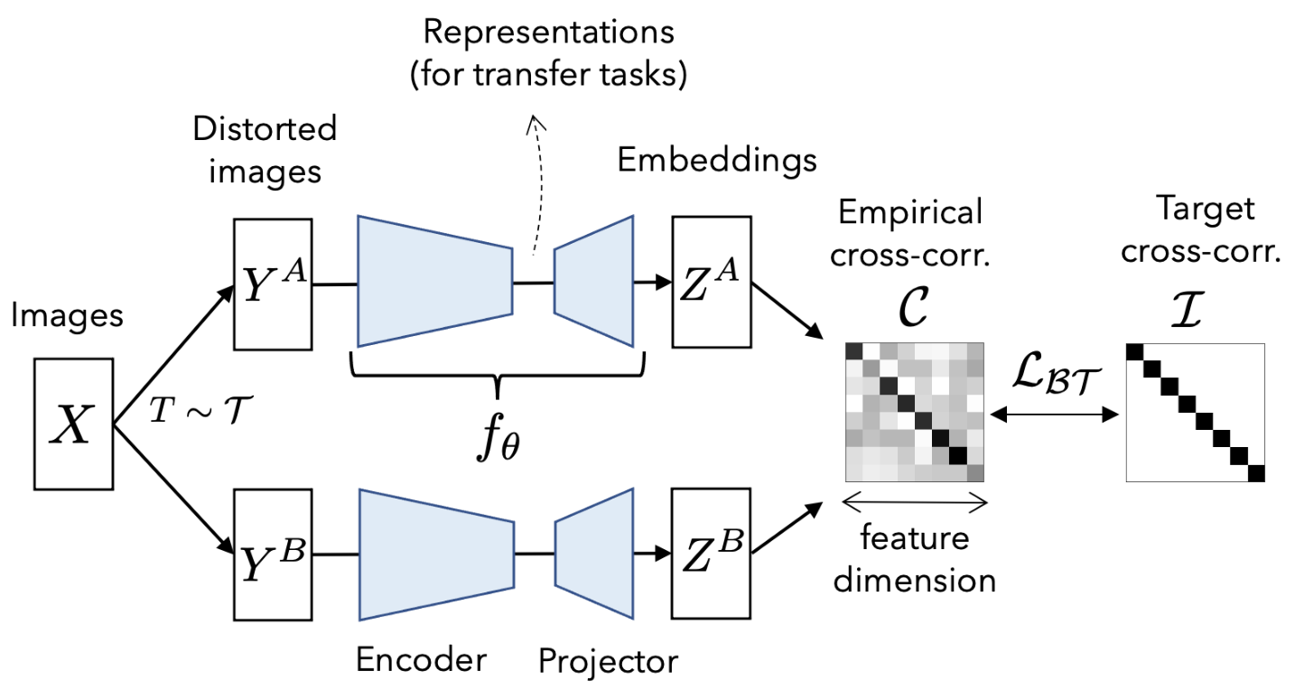
오른쪽 두 행렬은 경험적 cross-correlation C와 목표 identity I다. 축은 이미지 ID가 아니라 feature dimension이므로 N×N instance 비교표로 읽지 않는다. 대각은 같은 차원의 view 간 일치, 비대각은 차원 간 중복을 다룬다. 두 경로는 BYOL의 서로 다른 online·EMA target이 아니라 같은 network를 적용한 view들이며, downstream representation과 projection도 구별한다.
Jure Zbontar, Li Jing, Ishan Misra, Yann LeCun, Stéphane Deny · 2103.03230v3 · 원논문 · 원문 속 그림 · 크게 보기 원논문 도판 발췌. 지정한 PDF 버전에서 그림 영역만 잘라 고해상도 PNG로 렌더링했으며 내용을 다시 그리지 않았다. 한국어 해설은 별도 작성. 원권리자의 권리가 유지되며 블로그 코드의 MIT 라이선스가 도판 재배포 허락을 뜻하지 않는다.Batch를 B, projection 차원을 D라고 하면 두 표현은 B×D이고 correlation은 D×D다. 평균을 뺀 각 feature를 batch 축의 제곱합으로 정규화해 C_ij를 계산한다. 대각 항은 같은 feature가 view 간 일치하게 하고, 비대각 항은 feature 중복을 줄이려는 목적이다.
계산 예제. C=[[1,0.2],[0.2,1]], λ=0.005이면 diagonal cost=0, off-diagonal cost=0.005×(0.04+0.04)=0.0004다. i,j와 j,i를 둘 다 합산하는 정의에서 0.0002라고 쓰면 절반을 빠뜨린 것이다. C가 모두 0이면 diagonal cost는 D다. 다만 상수 feature의 분산이 0일 때 normalization 자체가 정의되지 않으므로 실제 구현의 ε 처리와 연결해 설명해야 한다.
논문의 평가와 ablation은 invariance 항·redundancy 항·projection 등의 효과를 검토한다. 이 loss의 모양만으로 모든 batch와 optimization에서 collapse가 절대 불가능하다는 일반 정리가 증명된 것은 아니다. 작은 batch의 상관 추정 품질과 zero-variance 처리는 구현에서 별도 시험한다.
#BYOL: target을 optimizer로 같이 움직이지 않는다
원본 Figure 2에서 online 경로는 encoder→projector→predictor, target 경로는 encoder→projector다. target representation에는 stop-gradient가 있고, target parameter는 online parameter의 EMA로 갱신한다. 서로 다른 증강 view의 역할을 바꾼 손실도 더한다. BYOL, 2006.07733v3, Figure 2 및 §3
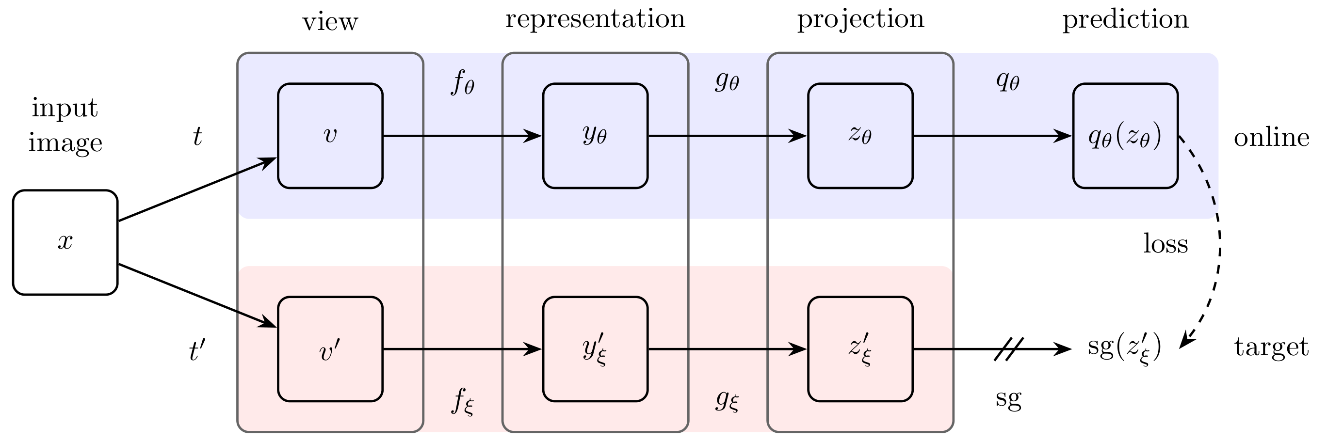
위쪽 prediction은 qθ(zθ), 아래쪽 target은 sg(z′ξ)다. 아래 경로의 sg는 그 방향 역전파를 끊는 표시이지 target parameter를 영원히 고정한다는 뜻이 아니다. EMA 갱신은 아래 식으로 따로 확인한다. 그림에는 한 방향만 그려져 있으며 대칭 손실은 두 view의 역할을 바꾸어 계산한다. 학습 후 representation으로 남기는 것은 online encoder의 yθ다.
Jean-Bastien Grill et al. · 2006.07733v3 · 원논문 · 원문 속 그림 · 크게 보기 원논문 도판 발췌. 지정한 PDF 버전에서 그림 영역만 잘라 고해상도 PNG로 렌더링했으며 내용을 다시 그리지 않았다. 한국어 해설은 별도 작성. 원권리자의 권리가 유지되며 블로그 코드의 MIT 라이선스가 도판 재배포 허락을 뜻하지 않는다.정규화한 prediction u와 target v의 제곱거리는 다음처럼 cosine과 연결된다. 이 식의 등식은 u와 v가 단위벡터일 때 성립한다.
계산 예제. cosine=0.8이면 한 방향 loss=0.4다. 반대 방향 cosine=0.6이면 loss=0.8이어서 두 방향 합은 1.2, 평균 convention이면 0.6이다. “두 방향”과 “loss reduction”을 구분한다. target의 이전 값이 0, online 값이 2, m=0.9이면 새 target은 0.2다. 이는 설명용 scalar 예이며 논문의 전체 parameter가 하나의 숫자라는 뜻이 아니다.
target을 optimizer parameter에 같이 넣으면 원래 stop-gradient 구조가 달라진다. 반대로 target을 영원히 고정하면 EMA 모델과도 다르다. 원문은 collapse 가능한 objective라도 실제 제안 구성에서는 유용한 학습을 관찰하고 bootstrapping·predictor 등의 ablation을 검토한다. EMA 하나만 있으면 어떤 모델도 collapse하지 않는다는 증명으로 확대하지 않는다. 원문의 ResNet-50 linear evaluation 74.3%도 데이터·학습 길이·평가 조건이 다른 다른 논문 숫자와 단독 모듈 기여로 빼지 않는다.
두 원본 구조도를 본문에 발췌해 loss·gradient 경로와 연결했다. 다만 구조도 자체가 collapse 방지를 모든 설정에서 보장하는 증명이나 ablation 결과표는 아니다. 모든 ablation 수치의 전사와 독립 학습 실험을 수행한 것은 아니다.
#8.6 memory bank와 MoCo
현재 batch의 view만 쓰면 비교 후보 수가 batch 크기에 묶인다. 과거 key를 저장하면 후보는 늘릴 수 있지만 encoder가 급격히 변할 때 오래된 key와 현재 query가 서로 다른 표현에 놓일 수 있다. MoCo는 큰 dictionary와 시간에 따른 일관성을 함께 다루려는 설계다. He 등, 1911.05722v3, §3
query encoder는 gradient로, key encoder는 이동평균으로 갱신한다. 이전 batch의 key를 queue에 보관해 많은 negative를 일관되게 쓴다.
#원본 Figure 1을 queue의 수명으로 읽기
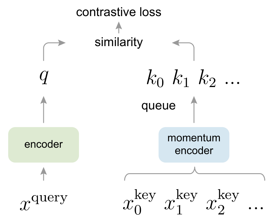
왼쪽 q를 오른쪽 encoded keys의 dictionary와 비교한다. queue가 유지하는 것은 key embedding이며, 새 mini-batch를 넣고 오래된 것을 빼는 수명 규칙은 본문으로 확인한다. 같은 점수 계산에 쓰이더라도 query의 gradient 학습과 key encoder의 momentum update는 다른 갱신이다. 이 overview는 queue의 모든 시간별 상태를 열거한 그림은 아니다.
Kaiming He, Haoqi Fan, Yuxin Wu, Saining Xie, Ross Girshick · 1911.05722v3 · 원논문 · 원문 속 그림 · 크게 보기 원논문 도판 발췌. 지정한 PDF 버전에서 그림 영역만 잘라 고해상도 PNG로 렌더링했으며 내용을 다시 그리지 않았다. 한국어 해설은 별도 작성. 원권리자의 권리가 유지되며 블로그 코드의 MIT 라이선스가 도판 재배포 허락을 뜻하지 않는다.MoCo 원본 Figure 1과 Figure 2에서 query, 이번 batch의 positive key, queue 안의 과거 key를 구분한다. 들어오는 key가 enqueue되고 오래된 key가 dequeue된다. queue에 저장하는 것은 원본 이미지가 아니라 계산한 key embedding이다. 그림의 queue를 단순한 이미지 재생 버퍼로 해석하면 메모리와 gradient 구조를 잘못 계산한다. 아래 Figure 1의 전체 흐름과 Figure 2의 gradient 비교를 함께 읽는다.
Query encoder는 gradient로 학습하고 key encoder는 느린 EMA 갱신을 사용한다. 과거 key embedding을 매번 최신 encoder로 다시 계산하는 것도 아니다. 그래서 “완전히 같은 encoder가 만든 key만 있다”보다 “encoder 변화가 완만하도록 해서 key들 사이의 불일치를 줄인다”가 정확한 설명이다.
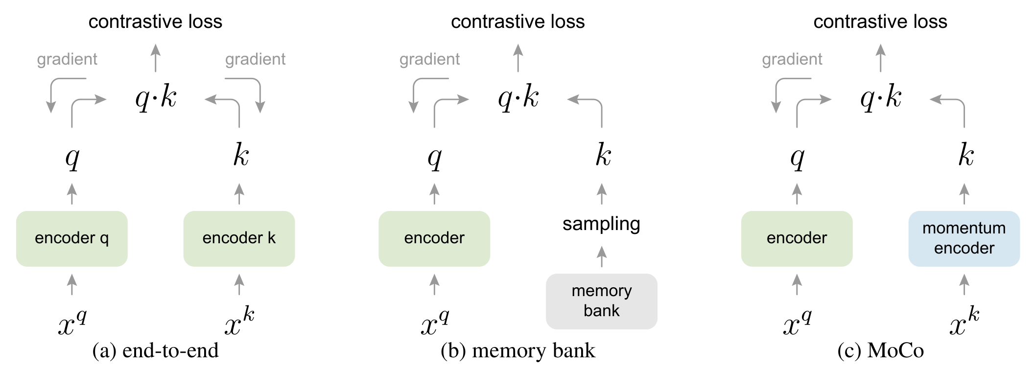
(a)는 두 encoder를 역전파로 갱신하고, (b)는 저장된 key를 memory bank에서 뽑으며, (c)는 새 key를 momentum encoder로 만든다. 원문 캡션은 queue가 이 Figure 2에는 그려지지 않았다고 명시한다. 없는 queue 화살표를 상상해 읽지 말고 Figure 1·본문과 연결한다. 세 구조의 개념 비교이지 이 그림 하나가 성능 격차의 수치 근거는 아니다.
Kaiming He, Haoqi Fan, Yuxin Wu, Saining Xie, Ross Girshick · 1911.05722v3 · 원논문 · 원문 속 그림 · 크게 보기 원논문 도판 발췌. 지정한 PDF 버전에서 그림 영역만 잘라 고해상도 PNG로 렌더링했으며 내용을 다시 그리지 않았다. 한국어 해설은 별도 작성. 원권리자의 권리가 유지되며 블로그 코드의 MIT 라이선스가 도판 재배포 허락을 뜻하지 않는다.해설용으로 query Q가 B×d, positive K+가 B×d, queue가 K×d이면 positive score는 B×1이고 negative score는 B×K다. 합친 logits는 B×(1+K)다. positive를 첫 열에 놓는 구현에서는 target index가 전부 0이지만, 이는 저장 순서에 따른 구현 convention이다.
#Queue 길이와 EMA의 기억 길이는 다르다
계산 예제. K=65536, batch=256의 전역 key를 매 step 넣으면 queue 한 바퀴는 256 step이다. 반면 m=0.999인 EMA에서 이전 parameter의 가중치가 절반이 되는 step 수는 다음과 같다.
256과 약 693은 서로 다른 메모리다. 하나는 저장된 embedding이 언제 교체되는지, 다른 하나는 parameter EMA에서 과거 상태의 영향이 얼마나 오래 남는지다. epoch 수로 바꾸려면 dataset 크기와 전역 batch를 추가로 알아야 한다.
m이 1이면 key encoder가 갱신되지 않고, m=0이면 query를 즉시 따라간다. 어느 극단이 좋을지는 학습 조건에 달려 있다. 원문은 dictionary 크기와 momentum에 관한 ablation을 통해 설계를 검토한다. 다른 MoCo 버전의 projection head·증강 변경을 섞어 “원형 MoCo”라고 쓰지 않는다.
#구현 순서가 loss를 바꾸는 경우
원형 연산을 따라 구현할 때는 현재 query와 positive를 계산하고, 이번 loss에서 사용할 과거 queue의 snapshot을 정한 뒤 score를 만든다. 새 key를 먼저 queue에 넣어 같은 positive가 negative 열에 다시 들어가면 분모의 의미가 달라질 수 있다. query의 gradient, no-grad key 계산, EMA timing, enqueue timing, distributed all-gather 뒤 global key 수를 명시한다.
MoCo의 shuffling BN은 batch statistics를 통한 shortcut을 줄이기 위한 장치다. 정답 pair를 무작위로 바꾸는 알고리즘이 아니며, key sample 순서를 다시 맞추는 단계가 필요하다. 오래된 queue의 tensor를 optimizer가 업데이트하는 parameter로 착각하지 않는다.
실험을 읽는 기준. MoCo는 frozen-feature linear classification뿐 아니라 detection·segmentation으로의 transfer를 평가했다. 좋은 linear top-1과 좋은 detector fine-tuning 결과는 같은 목표가 아니다. supervised pretraining과 비교할 때도 detector 구조, fine-tuning schedule과 초기 정규화 설정을 맞춘 표를 읽어야 한다. 이번 보강은 원리와 ablation의 질문을 설명하는 데 집중했고, detector별 표 전체의 수치 재전사나 실험 재현은 하지 않았다. MoCo, §4.1–4.2
#8.7 feature clustering: DeepCluster와 SwAV
#DeepCluster: 현재 표현에서 만든 label로 다음 표현을 학습하기
DeepCluster는 현재 feature를 clustering하고, 얻은 cluster assignment를 pseudo-label로 삼아 encoder를 학습하는 과정을 번갈아 수행한다. 원본 overview에서는 feature 추출→clustering→pseudo-label 학습이라는 반복을 읽는다. DeepCluster, 1807.05520v2, §3
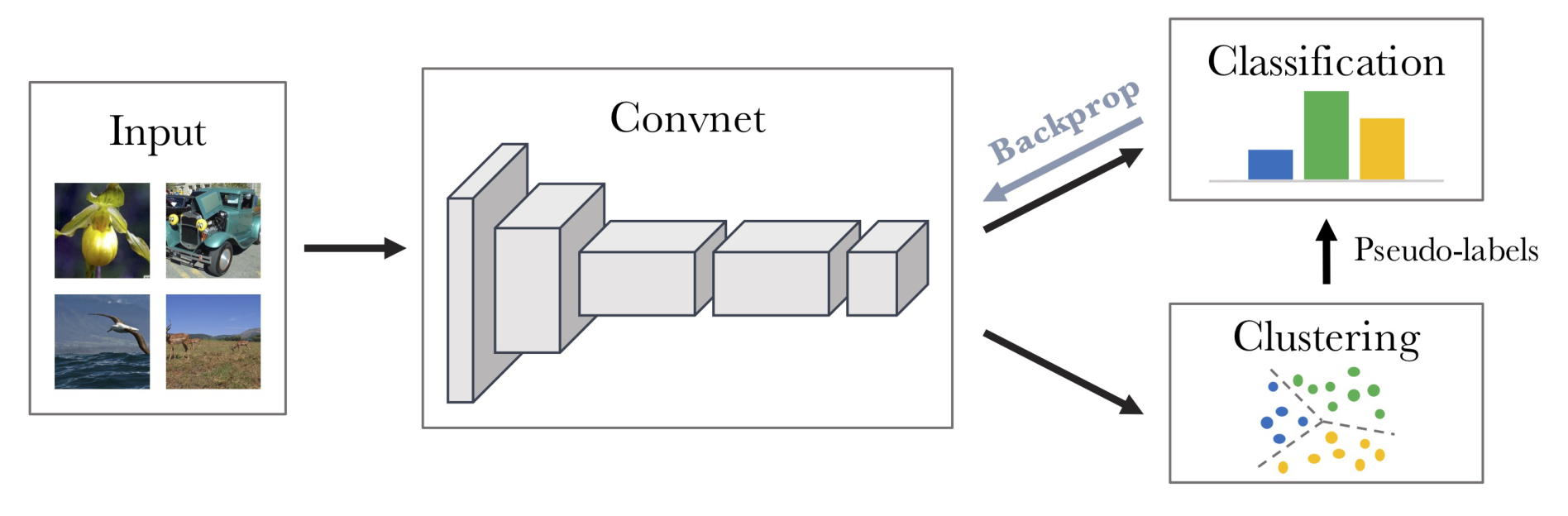
오른쪽 아래 clustering의 결과가 위 classification의 pseudo-label이 되고, 분류 학습의 역전파가 ConvNet을 갱신한다. cluster assignment를 만드는 단계와 고정한 pseudo-label로 학습하는 단계를 나누어 보자. 이 그림은 clustering의 이산 label 선택 전체를 하나의 미분 가능한 층으로 처리한다는 뜻이 아니며, cluster 번호가 의미 class 이름으로 고정된 것도 아니다.
Mathilde Caron, Piotr Bojanowski, Armand Joulin, Matthijs Douze · 1807.05520v2 · 원논문 · 원문 속 그림 · 크게 보기 원논문 도판 발췌. 지정한 PDF 버전에서 그림 영역만 잘라 고해상도 PNG로 렌더링했으며 내용을 다시 그리지 않았다. 한국어 해설은 별도 작성. 원권리자의 권리가 유지되며 블로그 코드의 MIT 라이선스가 도판 재배포 허락을 뜻하지 않는다.단순화한 k-means 단계는 아래와 같다. encoder가 고정된 동안 centroid와 assignment를 찾고, 다음 단계에서 assignment를 학습 목표로 사용하는 식으로 두 문제를 구분한다.
계산 예제. 1차원 feature [0,0.2,3,3.2]를 두 cluster로 나누면 centroid는 0.1과 3.1이다. 어느 cluster를 ID 0 또는 1로 부르는지는 바뀌어도 partition 자체는 같다. 다음 clustering에서 ID가 바뀌었는데 이전 classifier의 class 의미가 그대로라고 가정하면 안 된다. 한 cluster 쏠림과 빈 cluster를 처리하는 규칙도 필요하다.
실험은 clustering으로 얻은 표현의 downstream 전이와 설계 선택을 평가한다. pseudo-label이 실제 의미 class와 항상 일대일이라고 입증한 것은 아니다. 이번에는 알고리즘과 붕괴 위험을 설명했으며 논문의 개별 downstream 수치표를 모두 재구성하지는 않았다.
#SwAV: 한 view의 assignment로 다른 view의 prototype prediction을 학습
SwAV는 prototype에 대한 assignment를 서로 다른 view 사이에서 교환해 예측한다. 모든 instance pair의 negative를 직접 비교하는 것과 다르다. 원본 Figure 1에서 두 view의 예측과 assignment가 서로 엇갈려 supervision을 제공하는 흐름을 따라간다. SwAV, 2006.09882v5, §3
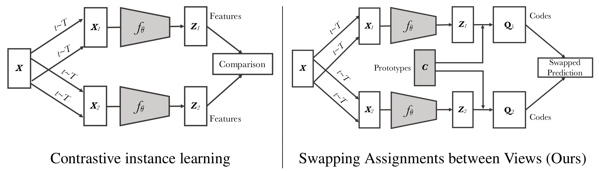
오른쪽의 C는 prototypes, q1·q2는 각 view의 code다. 한 view에서 얻은 code를 다른 view의 prediction에 주는 교차 감독이 핵심이며, 왼쪽처럼 두 feature의 similarity만 직접 높이는 연산으로 줄일 수 없다. assignment를 구하는 제약과 prediction의 cross entropy를 구분해야 아래의 Q 질량 정규화 식이 왜 필요한지 이해할 수 있다.
Mathilde Caron, Ishan Misra, Julien Mairal, Priya Goyal, Piotr Bojanowski, Armand Joulin · 2006.09882v5 · 원논문 · 원문 속 그림 · 크게 보기 원논문 도판 발췌. 지정한 PDF 버전에서 그림 영역만 잘라 고해상도 PNG로 렌더링했으며 내용을 다시 그리지 않았다. 한국어 해설은 별도 작성. 원권리자의 권리가 유지되며 블로그 코드의 MIT 라이선스가 도판 재배포 허락을 뜻하지 않는다.D차원 embedding N개와 K개 prototype이면 prediction matrix는 N×K다. balanced assignment를 계산하는 과정의 정규화된 질량행렬을 Q∈R^(K×N)로 두면 다음 같은 marginal 제약을 사용한다. sample별 확률로 쓸 때에는 Q의 각 열을 N배 해 열 합이 1이 되게 만드는 convention을 구분한다.
계산 예제. K=N=2에서 Q가 diagonal 원소 0.5, 나머지 0이면 총 질량은 1이고 두 제약을 만족한다. Q 자체의 각 열 합은 0.5이지 1이 아니다. 반면 2Q는 각 표본의 one-hot assignment가 된다. 이 둘을 혼동하면 cross entropy weight가 batch 수에 따라 잘못 변한다.
두 view A,B의 assignment를 qA,qB, prediction을 pA,pB라고 하면 한 쌍의 swapped loss는 아래와 같다. 본문의 기호를 재정리한 표현이다.
이 균형 제약은 prototype 사용을 조절하는 학습 장치이지 실제 세계의 class 빈도가 균등하다는 증거가 아니다. 원문은 online clustering·multi-crop 등의 설정을 실험한다. 모든 향상을 “negative가 없어서”라고 한 가지 원인으로 돌리지 않는다. 여기서는 핵심 objective와 질량 보존을 보강했고 Sinkhorn의 수치 안정성과 전체 ablation은 추가 심화 대상이다.
#8.8 label이 일부 있다면: supervised contrastive learning
SupCon에서는 anchor와 같은 class인 sample들을 positive 집합으로 사용한다. label이 없는데도 진짜 같은 class를 자동으로 알 수 있다는 가정이 아니다. SupCon, 2004.11362v5, §3
원문의 주요 형태에서는 positive별 log 확률의 평균을 사용한다. positive의 확률들을 먼저 평균내고 log를 취하는 것과 다르다. 분모의 비교 집합에서는 anchor만 제외하며 다른 positives는 남는다.
계산 예제. 두 positive의 softmax 확률이 0.2와 0.6이라고 하자. negative log의 평균은 1.060132, 평균 확률의 negative log는 0.916291이다. 한 positive만 매우 높고 다른 positive가 낮을 때 두 목적은 다른 벌점을 준다.
Label이 일부만 있는 batch에서 유효 positive가 없는 anchor를 어떻게 처리할지도 정해야 한다. 분모가 0인 집합 크기로 나누지 않도록 하고, distributed batch에서는 positive mask와 sample ordering을 맞춘다. 논문의 결과는 supervised representation 학습의 효용을 보여 주지만 class 내부의 모든 다양성을 없애는 것이 언제나 최선이라는 뜻은 아니다. 여기서는 objective 비교까지 보강했으며 모든 backbone별 최고 점수표를 새로 전사하지 않았다.
#8.9 CLIP: positive를 image–text pair로 확장
CLIP은 같은 이미지의 두 증강만이 아니라 이미지와 text의 짝을 학습한다. 학습 뒤에는 label 설명을 text encoder에 넣어 이미지와 비교한다. 이미지 설명 문장을 생성하는 autoregressive decoder와는 다른 연산이다. 참고 버전은 Radford 등 2103.00020v1이다. CLIP, §2, Figure 1
batch의 N개 image와 N개 text 사이 N×N similarity matrix를 만들고, 올바른 대각 쌍이 커지도록 양방향 cross entropy를 학습한다.
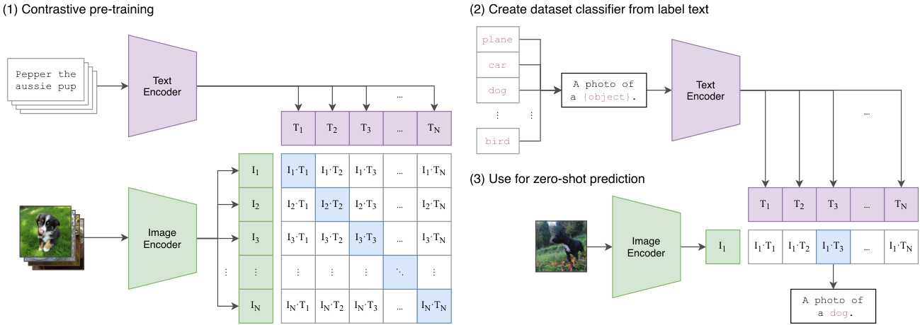
왼쪽 큰 표는 학습용 image–text similarity matrix다. 대각의 짝이 supervision이다. 오른쪽 위는 label text로 classifier의 비교 벡터를 만드는 과정이고, 오른쪽 아래는 새 영상과 그 벡터들의 비교다. 학습 batch의 captions와 추론 시 class prompts를 혼동하지 않는다.
Alec Radford et al. · 2103.00020v1 · 원논문 · 원문 속 그림 · 크게 보기 원논문 도판 발췌. 원문 PNG 파일을 그대로 사용했다. 한국어 해설은 별도 작성. 원권리자의 권리가 유지되며 블로그 코드의 MIT 라이선스가 도판의 재배포 허락을 뜻하지 않는다.#두 encoder와 양방향 cross entropy
같은 차원으로 투영하고 정규화한 image embedding I, text embedding T가 각각 N×D라면 logits는 N×N이다. 학습 가능한 log scale을 t라고 쓰면 아래처럼 나타낼 수 있다. t를 그대로 temperature라고 부르지 않는다. exp(t)는 inverse temperature 역할의 logit scale이다.
행에서는 각 이미지의 정답 text를, 열에서는 각 text의 정답 이미지를 찾는다. 두 방향의 평균을 쓰는 convention이다. SimCLR처럼 대각을 self-similarity라 생각해 지우면 안 된다. CLIP 대각은 정답 image–text pair다. 행마다 N개 후보 중 하나가 positive이므로 negatives는 N−1개다.
계산 예제. 두 쌍의 logits를 [[2,0],[0,2]]로 두면 각 방향의 loss는 log(1+exp(−2))≈0.126928이다. 두 방향 평균도 같은 값이다. 대각을 mask하면 학습할 정답을 삭제하게 된다. 이 예의 logit 2는 설명용 값이며 실제 pretrained CLIP의 temperature를 주장하는 숫자가 아니다.
#Zero-shot classifier의 shape를 다시 따라가기
추론할 이미지 B개와 후보 class K개가 있으면 image feature는 B×D, label prompt feature는 K×D다. 둘을 곱한 결과는 B×K다. 학습 batch N과 test-time class 수 K는 같을 필요가 없다. class 이름을 문장 template에 넣는 이유와 여러 prompt를 평균할 때 정규화하는 위치도 명시한다.
예를 들어 text 후보가 dog와 cat뿐인 분류에서 dog score가 높은 것과, dog·cat·wolf·fox·bear를 함께 둔 분류에서 dog 확률이 높은 것은 같은 조건이 아니다. softmax 확률은 후보 집합에 의존한다. “가장 비슷한 문장”을 찾는 점수와 절대적으로 보정된 인식 신뢰도는 구분한다.
논문이 검토한 것과 검토하지 않은 것. CLIP은 대규모 image–text pretraining과 여러 downstream 데이터셋의 zero-shot·linear-probe 등을 비교했다. zero-shot은 해당 target task의 학습 label로 classifier를 fitting하지 않는 protocol을 뜻하지, 사전학습 데이터·자연어 supervision·bias가 없다는 뜻이 아니다. 원문은 prompt engineering과 dataset shift의 영향도 다룬다. CLIP, §3
SimCLR linear-probe top-1과 CLIP zero-shot top-1을 놓고 “표현 품질만의 차이”라고 단정하지 않는다. supervised head의 유무, pretraining 데이터, backbone, image resolution, text prompt가 함께 달라진다. 새로운 task에서 prompt를 test set에 반복 맞추었다면 zero-shot이라는 말만으로 평가 독립성이 유지되지 않는다. 이것은 평가 설계상의 주의이며 원문이 모든 실제 배포에서 calibration을 보장했다는 주장이 아니다.
#8.10 방법을 고르는 기준
| 상황 | 우선 볼 방법 | 핵심 검증 질문 |
|---|---|---|
| 한 batch의 두 view를 대조 | SimCLR | positive 포함 분모, self mask, h/z 구분이 맞는가 |
| 작은 batch와 큰 dictionary | MoCo | queue 수명, EMA timing, key의 gradient가 맞는가 |
| explicit negative를 피함 | BYOL·Barlow Twins | target 갱신·stop-gradient·correlation 축이 맞는가 |
| 반복되는 prototype 학습 | DeepCluster·SwAV | assignment의 의미·균형·질량 정규화가 맞는가 |
| label을 positives에 반영 | SupCon | positives 평균을 log 밖에서 하는가, 빈 집합 처리는 무엇인가 |
| image–text zero-shot 비교 | CLIP | 대각을 정답으로 두는가, task label fitting과 구분하는가 |
이 표는 새 benchmark 순위가 아니라 읽기와 구현의 점검표다. 논문별로 positive/negative 정의, 저장하는 tensor, gradient 경로, loss의 합·평균, pretraining과 downstream의 데이터 사용을 적으면 같은 “대조학습” 이름 뒤에 숨어 있는 실제 차이가 보인다.