Self-Improving AI 01 — What Changes When AI Gets Better? distinguished the target of change, the scope of automation, and the evaluation criteria. We now follow the process that trains model parameters.
#Slide 6 — How does AI learn?
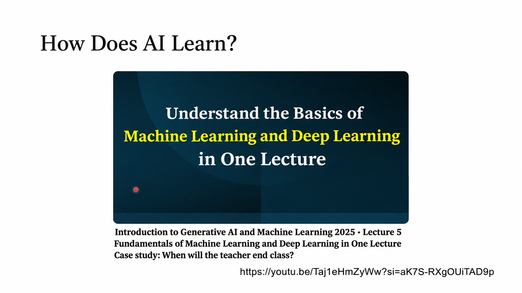
Original slide 6 · Video at approximately 03:37–04:01
This transition slide reviews machine learning before introducing self-improvement. The central thumbnail points to the instructor’s fifth lecture in the 2025 introductory course.
To understand self-improvement, first identify what changes in ordinary training. For illustration, write a model as follows.
- : the input.
- : the model specified by parameters .
- : the model’s output.
- : trainable values, such as weights and biases.
In estimating human joint positions from an image, for example, is the image and gives the joint coordinates. A language model takes an input context, computes a distribution over the next token, and builds a sentence by choosing successive tokens from these distributions.
Inference computes an output with a given model. Parameter learning changes according to a specified criterion. From this slide onward we focus on the latter.
The question about self-improvement now becomes more precise.
Can AI produce the training data or targets that change a model? If so, how can we judge the quality of those targets?
Slide 7 breaks the question into three parts.
#Slide 7 — The objective, candidates, and optimization
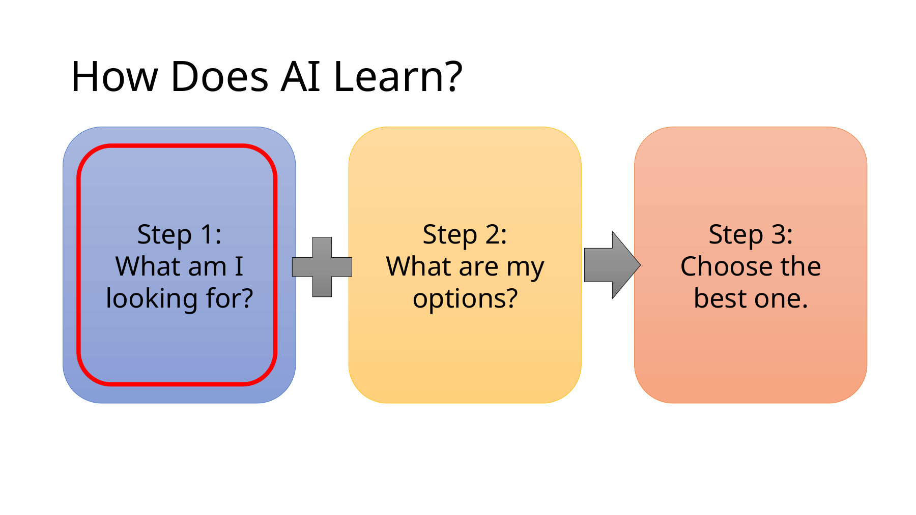
Original slide 7 · Video at approximately 04:01–04:56
The diagram distinguishes what we seek, the available choices, and the procedure for choosing a good one. A red border around the first blue box marks the particular focus of this lecture.
Here is that distinction in machine learning terms.
| Question on the slide | Machine learning concept | Joint position estimation example |
|---|---|---|
| What are we looking for? | Problem definition and criteria for a good output | Output coordinates close to the ground-truth joints in the image |
| What choices are available? | Hypothesis space, the set of functions the model can express | The selected network architecture and possible parameter values |
| How do we select a good choice? | Optimization | Compute a loss and update parameters using gradient descent or another optimizer |
#Model architecture and training objectives play different roles
Even with the same network architecture, different values of produce different functions. Write the candidate set as follows.
Here is the set of allowed parameter values, and is the set of functions those values can express.
A loss function evaluates how well a candidate model performs. The ideal objective of finding the best parameters under this criterion can be written as follows.
A training algorithm searches candidates in pursuit of this objective. The basic gradient descent update is
- : the learning rate, which sets the step size.
- : the gradient, pointing in the direction of increasing loss at the current position.
- The minus sign specifies a step in the opposite direction to reduce the loss.
This equation does not guarantee a global minimum for every neural network. Initialization, data, model architecture, and optimizer settings all influence the solution. A good candidate on training data also requires separate evaluation for generalization to new data. Supplement: Stanford CS229 notes on supervised learning and gradient descent
#Supplementary lecture · Stanford CS229 — What value does optimization change?
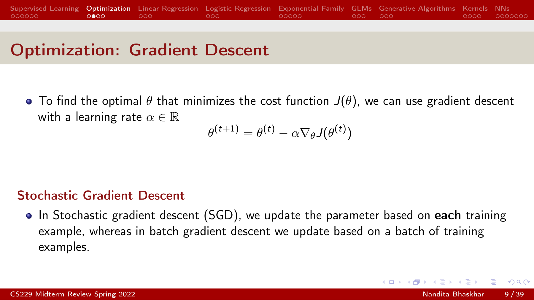
On the Stanford slide, corresponds to our total loss , and learning rate to . The update changes parameter . The discussion of stochastic gradient descent (SGD) below it distinguishes which training examples contribute to a single update.
Compare the equation with the first box on the NTU slide. If a different teacher supplies different target labels, the same gradient descent algorithm may receive a different loss and gradient. Examine both the optimizer and the target it receives.
#Why highlight the first box?
In self-improvement, the model architecture is only one possible target of change. AI can also generate or propose the data, answers, rewards, and losses that define a good answer.
For example, even with the same model and optimizer, the following training procedures differ.
- Use human-reviewed joint coordinates as targets.
- Use joint coordinates predicted by an existing model as targets.
The search procedure may stay the same while changing what the model learns to approximate. This distinction runs through slides 8–10.
#Slide 8 — The difference between the output and the target provides a learning signal
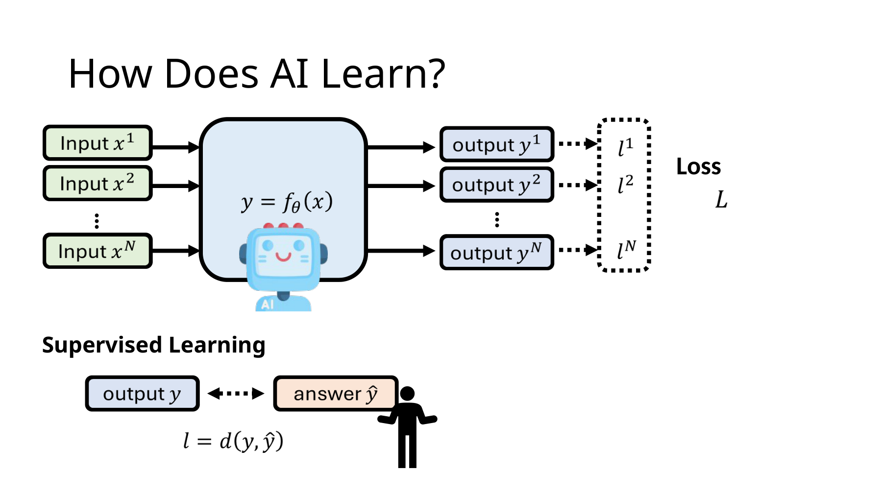
Original slide 8 · Video at approximately 04:56–07:02
In this figure, is the model output, and is the correct answer or training target. Other texts use for a prediction, so check the role of each symbol here.
#Reading the diagram from left to right
The same model maps inputs to outputs . Superscript indexes examples rather than raising a value to a power.
Compute an individual loss from the discrepancy between each output and its corresponding target.
Here evaluates the discrepancy. It need not be a mathematical metric satisfying symmetry and the triangle inequality.
Denote the overall loss aggregating individual losses by .
Define a good output for an individual example, then adjust parameters to satisfy that criterion across the data.
#A numerical regression loss example
Consider a hypothetical distance prediction task measured in meters, with squared error as the individual loss.
| Example | Target | Model A output | A squared error | Model B output | B squared error |
|---|---|---|---|---|---|
| 1 | 1.0 | 1.2 | 0.04 | 1.1 | 0.01 |
| 2 | 2.0 | 1.9 | 0.01 | 2.5 | 0.25 |
| Total | 0.05 | 0.26 |
B is more accurate on the first example. A does better under the criterion aggregated across both.
For mean squared error (MSE), divide the sum by . A’s MSE is 0.025 and B’s is 0.13. On the same fixed data, sums and means rank models identically but give gradients of different magnitudes. Read the learning rate alongside the loss definition in implementations.
#Cross-entropy for classification
If denotes the probability assigned to the correct class, a common loss is
In a hypothetical example using natural logarithms, a probability of 0.8 for the correct class produces a loss of approximately 0.223, while 0.2 yields about 1.609. Unlike accuracy, which counts correct final choices, the loss responds to changes in the probability assigned to the correct class. Supplement: classification and logistic regression in CS229
So far the target has been given. Next we change who fills in the answer box at the bottom of the diagram.
#Slide 9 — Knowledge distillation from a strong AI’s answers
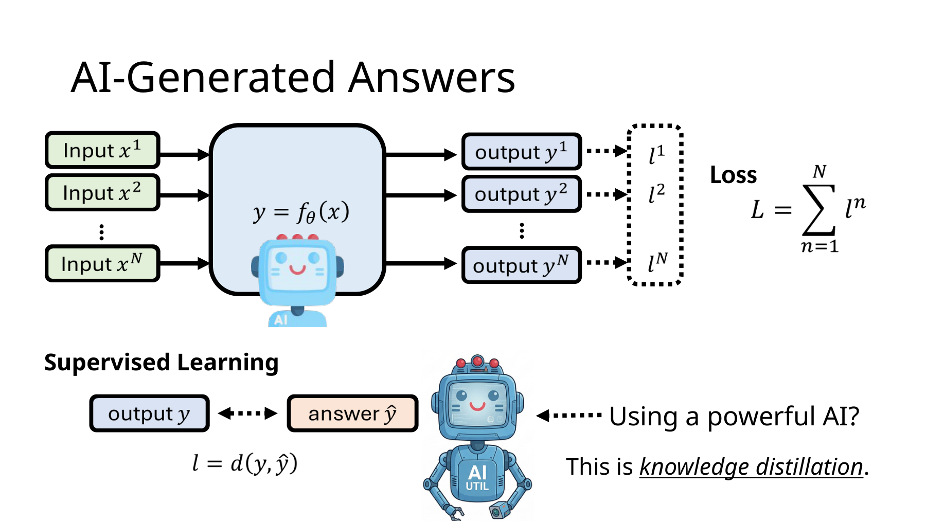
Original slide 9 · Video at approximately 07:02–08:03
Compared with the previous slide, a strong AI with a different appearance now stands beside the lower answer box. It supplies the training targets. The lecture introduces this as knowledge distillation.
The model that teaches is the teacher, and the one that learns is the student. Training moves the student’s outputs toward the teacher’s targets.
#Transferring an answer or a probability distribution
Start with the answer box on the slide. The teacher produces answer to question . We introduce to distinguish the AI-generated target. It occupies the position labeled on the slide.
One loss for a language model learning from that answer is
The probability of an entire sentence is a product of token-level conditional probabilities. Taking its negative logarithm gives a sum of token losses.
Another approach uses the teacher’s output distribution as the target. For class , let be the teacher distribution and the student distribution.
The teacher distribution is a fixed target during the student update. Both approaches use the teacher’s output, but they communicate different information. Hinton and colleagues’ 2015 paper describes distillation using output distributions and temperature. Original paper, section 2
#Supplementary lecture · Lambert — Fix the teacher distribution and update the student
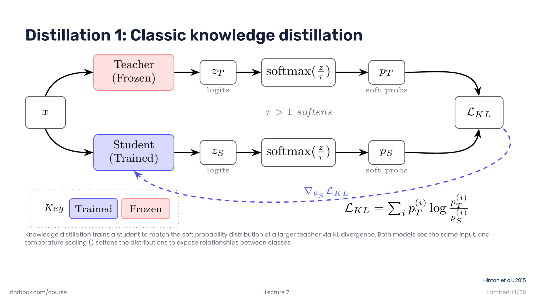
The upper teacher is labeled Frozen and the lower student Trained. Both receive the same input, but the gradient along the dashed arrow changes only the student. Updating the teacher’s target would move what the student is trying to match, so the diagram holds the teacher distribution fixed.
Temperature in the middle adjusts how sharp the distribution is when logits become probabilities. The setting reveals information beyond the largest probability. This differs from supplying a completed answer as a target. The student matches the teacher’s distribution across possibilities.
#What extra information does the distribution retain?
Consider a hypothetical three-class example.
| Target representation | Class A | Class B | Class C |
|---|---|---|---|
| Target retaining only the most probable class | 1.0 | 0.0 | 0.0 |
| Teacher’s soft target | 0.7 | 0.2 | 0.1 |
Both targets identify A as the most likely class. The soft target also records that the teacher considered B a more plausible alternative than C. The student can learn these relative relationships.
The teacher distribution can contain errors. Receiving a detailed distribution does not by itself make it a correct target.
#Must a “strong teacher” be a larger model?
Distillation extends beyond compressing a large model into a small one. What matters is what supplies a better learning signal. Noisy Student studies students of equal or greater size and introduces noise during training. Distinguish model size from the quality of the teacher’s signal. Noisy Student, CVPR 2020
A different teacher supplies the target on this slide. Slide 10 puts the model being trained in that teacher’s place.
#Slide 10 — Can a model teach itself with its own answer?
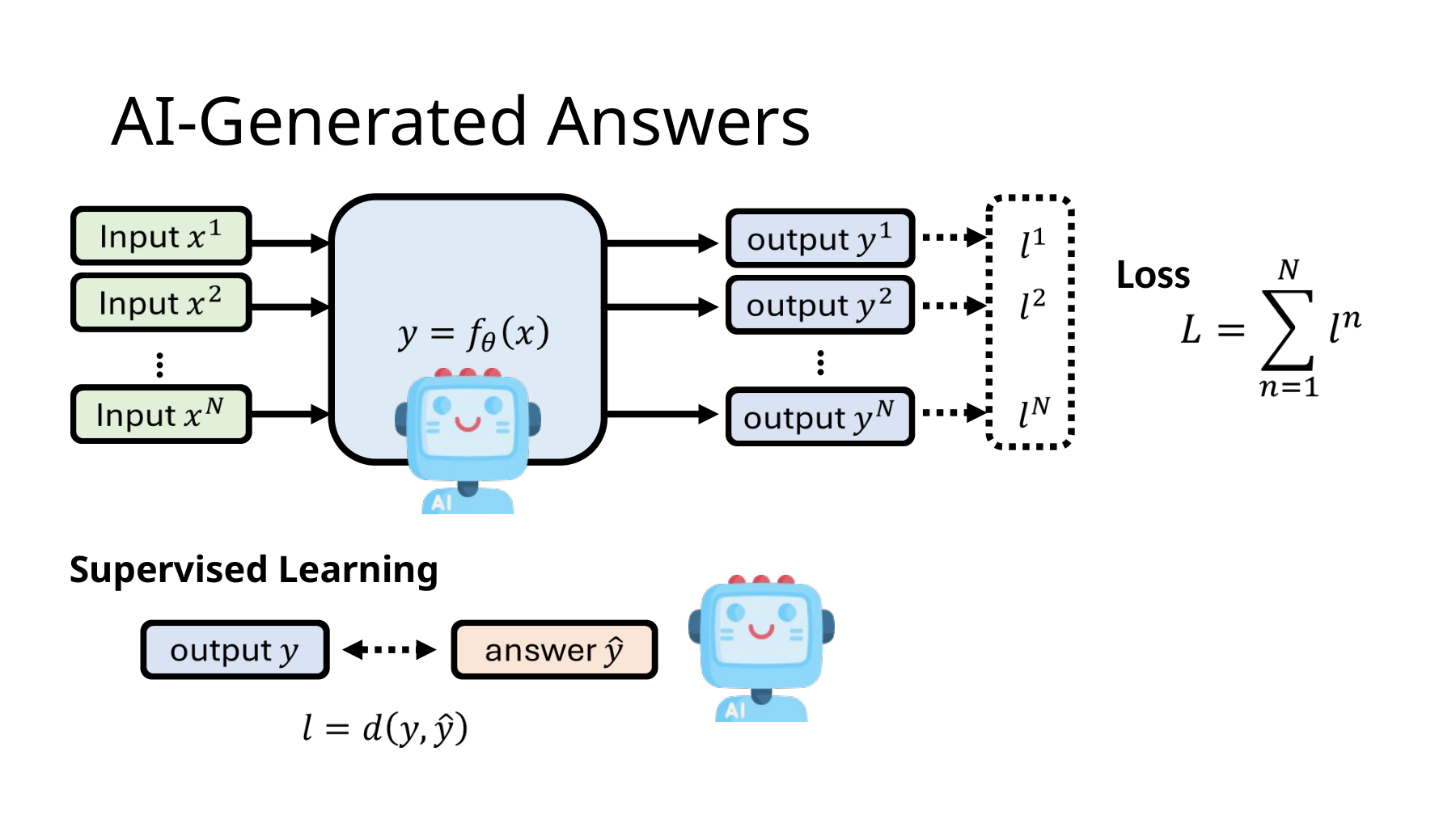
Original slide 10 · Video at approximately 08:03–08:31
The most visible change is that the teacher robot below now looks like the model being trained above.
The slide asks whether self-generated pseudo-answers can serve as training targets. A pseudo-answer is a target assigned for training. Its correctness has yet to be established.
When a model learns from its own output, first ask which form of output becomes the target.
#Case A. Matching the model’s own probability distribution directly
Let be the model’s current weights. Use the distribution obtained on the same input as a fixed target.
Stop-gradient means derivatives do not flow through the target-producing branch. Suppose the student starts at and that identical inputs, temperatures, and execution conditions produce exactly identical distributions.
At temperature 1, the gradient of cross-entropy with respect to student logit is
When both distributions agree,
This distillation loss itself supplies no learning direction. The result follows by substituting identical distributions into the logit gradient. Hinton et al., 2015, section 2
All assumptions matter. Dropout or input augmentation may make the distributions differ. A separate ground-truth loss or regularization term can also change the result. Optimizer momentum or weight decay may still move parameters, so the claim here concerns only the gradient of this distillation loss.
Also, zero gradient and zero loss are different conditions.
With identical distributions, their cross-entropy still equals the distribution’s entropy. For example, gives cross-entropy of approximately 0.5004. That remaining value does not give the student a further direction to move.
#Supplementary lecture · Lambert — What decreases in cross-entropy?
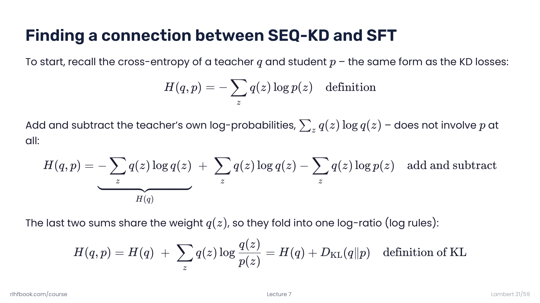
The slide’s is our . The last line separates it into the teacher’s uncertainty and KL divergence measuring the difference between the distributions. With a fixed teacher, only the KL term can change through student updates.
The residual after the distributions agree is therefore not unresolved student error. Treating KL as the only reducible term requires a fixed teacher. Recomputing the teacher with the same parameters and differentiating through that branch would optimize a different objective.
#Case B. Turning a prediction into one hard label
Consider a hypothetical defect classifier that predicts a defect probability of 0.8. Based on this prediction, assign the pseudo-label “defective,” or .
In binary cross-entropy, the gradient with respect to defect logit is
Gradient descent increases the logit. In a calculation directly updating one logit, with and learning rate ,
A learning signal arises even though it originated from the same model’s prediction. The procedure changed the probability target into hard label .
If the item is actually normal, the model has become more confident in an incorrect judgment. An increase in predicted probability and an increase in actual accuracy require separate checks. A model score of 0.8 does not guarantee 80% empirical correctness.
This calculation illustrates the movement of one logit. Real networks share weights across inputs, so we cannot infer that outputs for all examples change the same way.
#In depth. What if we train on every randomly generated answer?
Making the most likely answer a hard label differs from randomly sampling an answer from the model distribution. Suppose we fit all sampled answers by maximum likelihood without selection.
Under that sampling distribution, the expected gradient at the starting point is
This follows from probabilities summing to one when the output space is fixed and differentiation can be exchanged with summation.
A finite sample can give a nonzero gradient. Movement due to sampling alone, however, is insufficient evidence of a signal pointing toward the correct answer. This observation does not rule out all effects over multiple actual training rounds.
#What changes in actual self-training?
Research using self-generated data changes the target-generation procedure, the data, or the conditions under which the student learns.
| What changes | Why the learning signal changes |
|---|---|
| Filter generations using answers, tests, or rewards | The distribution of outputs retained for training changes |
| Augment student inputs | The student learns the teacher’s target across different observations of the same content |
| Add noise to the student | The student runs under different conditions from the teacher that produced the targets |
| Add new unlabeled inputs | Training constrains input regions previously unseen |
| Change the student’s initialization, capacity, or training procedure | The same signal can be represented by different functions and optimization paths |
Three original studies illustrate these possibilities.
Noisy Student, CVPR 2020. A teacher assigns pseudo-labels to unlabeled images, and a student trains on both labeled and pseudo-labeled data. The student uses data augmentation and model noise and may be as large as or larger than the teacher. Original paper
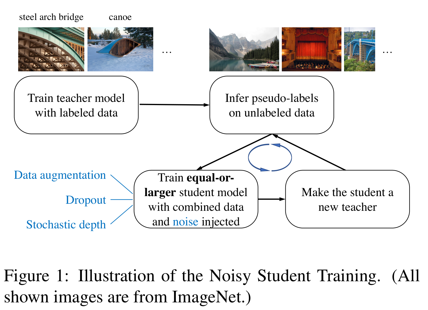
The upper-left teacher starts with labeled data and then labels unlabeled inputs. The student below uses both kinds of data. Data augmentation, dropout, and stochastic depth, marked in blue, apply during student training. The teacher turns these sources of noise off when generating pseudo-labels.
The figure differs from matching the same distribution on identical inputs under identical execution conditions: it adds new inputs and changes the student’s training conditions. The final arrow reuses the trained student as the next teacher. That arrow alone does not establish improvement, which requires separate evaluation.
STaR, NeurIPS 2022. STaR trains on generated rationales that reach a correct answer. After a failure, it regenerates a rationale conditioned on the correct answer. Problems, answers, and initial worked examples enter the procedure. Original paper
ReST, August 2023. ReST separates Grow, which generates data, from Improve, which trains on data filtered by reward. The paper considers negative log-likelihood and several offline reinforcement learning losses, so the method extends beyond a single loss. Original paper, section 3
None of these ingredients guarantees improvement. Incorrect pseudo-labels, inaccurate selection criteria, or augmentations that change a label’s meaning can cause problems. Check the direction of change and the outcome on new data.
The question on slide 10 can now be phrased more precisely.
What new learning signal was constructed from the model’s outputs, and how did the experiment establish that the signal improves the desired capability?
Next, Self-Improving AI 03 — When Does Self-Correction Become Learning? covers self-correction beginning on slide 11. It distinguishes revising an answer from using the revised answer as training data to update parameters.
#Further reading
Lecture PPTX · PDF · Lecture video
- Hung-yi Lee, official NTU ML 2026 course. Self-Improving, Part 1, PDF pages 6–10: learning targets and AI-generated answers.
- Stanford CS229 lecture notes. Foundations of supervised learning, gradient descent, and classification losses.
- Nandita Bhaskhar, Stanford CS229 Midterm Review. May 6, 2022. PDF page 9: parameter updates in gradient descent.
- Hinton, Vinyals, Dean, Distilling the Knowledge in a Neural Network. March 9, 2015. Knowledge distillation using probability distributions.
- Xie et al., Self-training with Noisy Student improves ImageNet classification. CVPR 2020, arXiv v4 (June 19, 2020). Figure 1 on PDF page 2: iterative teacher–student training.
- Zelikman et al., STaR: Bootstrapping Reasoning With Reasoning. NeurIPS 2022. Filtering and learning from generated rationales.
- Gulcehre et al., Reinforced Self-Training (ReST) for Language Modeling. arXiv v2 (August 21, 2023). Iterating generation, selection, and training.
- Nathan Lambert, Post-training Course, Lecture 7 · Official PDF. PDF page 14: teacher–student distillation. Page 21: the relationship between cross-entropy and KL divergence.