An agent’s prompts and model weights can both change. Updating both does not guarantee a gain. The outcome depends on which component is optimized first, which score guides selection, and whether the result holds when the goal changes.
Episode 17 examined agent code, archives of candidates, DSPy programs, and models that retrieve past experience. Pages 21–25 of the second lecture ask a further question. How does improving external components such as memory and instructions interact with training the weights θ directly?
Worked examples Retrieval and accuracy · E-SPL selection · Inspection costs
Video and papers by slide
| Slide | Lecture and related material | Question |
|---|---|---|
| Part II, p. 21 | 21:00 · ExpRAG paper | What changes when we train the model that reads the retrieved experience? |
| Part II, p. 22 | 22:11 · BetterTogether paper | Does the order of prompt and weight updates matter? |
| Part II, p. 23 | 24:15 · DSPy lecture slides | Can we apply gradient descent directly to a harness? |
| Part II, p. 24 | 24:35 · E-SPL paper | What roles do evolution and reinforcement learning play? |
| Part II, p. 25 | 25:19 · Original PDF | Should the previous best candidate still be used when the goal changes? |
Each time link opens the spoken explanation for that concept. The times follow the start of the corresponding cue in NTU’s Traditional Chinese caption track.
#Part II, p. 21 — Retrieve a memory, then train the model to use it
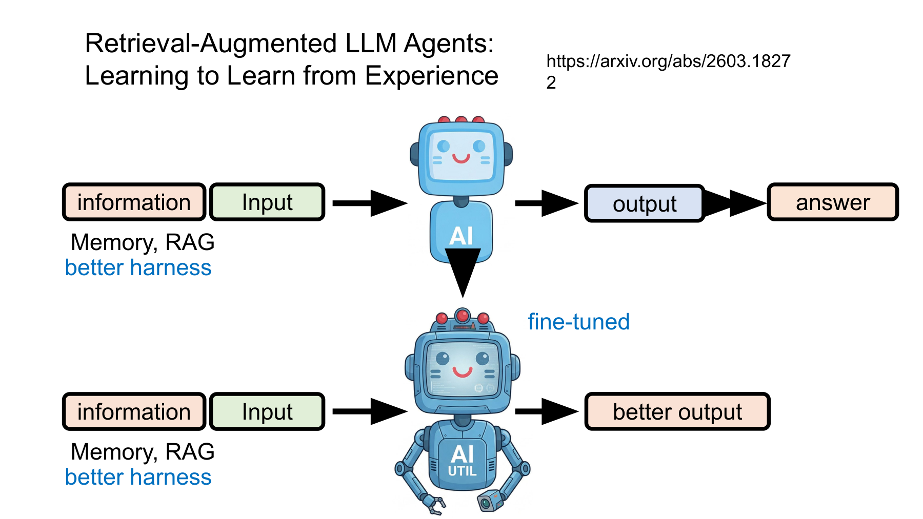
This slide extends the side-by-side comparison on page 20. The upper path, information and input → AI → output → answer, depicts retrieval-augmented generation (RAG). Past documents enter as external input. The lower arrow adds fine-tuning so the model can make better use of the same information and input.
#What changes during retrieval and training?
| Mechanism | What changes | Possible without training? | Possible failure |
|---|---|---|---|
| RAG or memory retrieval | The index, top K, and assembled context in h | Yes | Irrelevant experience, long context, stale information |
| Fine-tuning | Weights θ or LoRA adapters | No | Overfitting, training-data leakage, regression on earlier capabilities |
| Training to use retrieved experience | The interaction between learned θ and retrieved context h | Training required | Memorizing experience patterns seen only in training |
ExpRAG stores execution trajectories in an Experience Bank. For a new problem it retrieves the top K relevant experiences and supplies them to an LLM policy. The research question is whether the model interprets the retrieved experience well enough to change its actions. Retrieval quality and the ability to use the results require separate measurements. ExpRAG, EMNLP 2026
The following notation illustrates the distinction and abstracts away implementation details of the paper.
The first equation adds information during inference. The second produces a new model trained to use that kind of input. Training can also hurt performance. To compare systems, hold the retrieval index and evaluation set fixed and record token costs and whether retrieval was enabled.
#DSPy lecture — A RAG program has more than one parameter
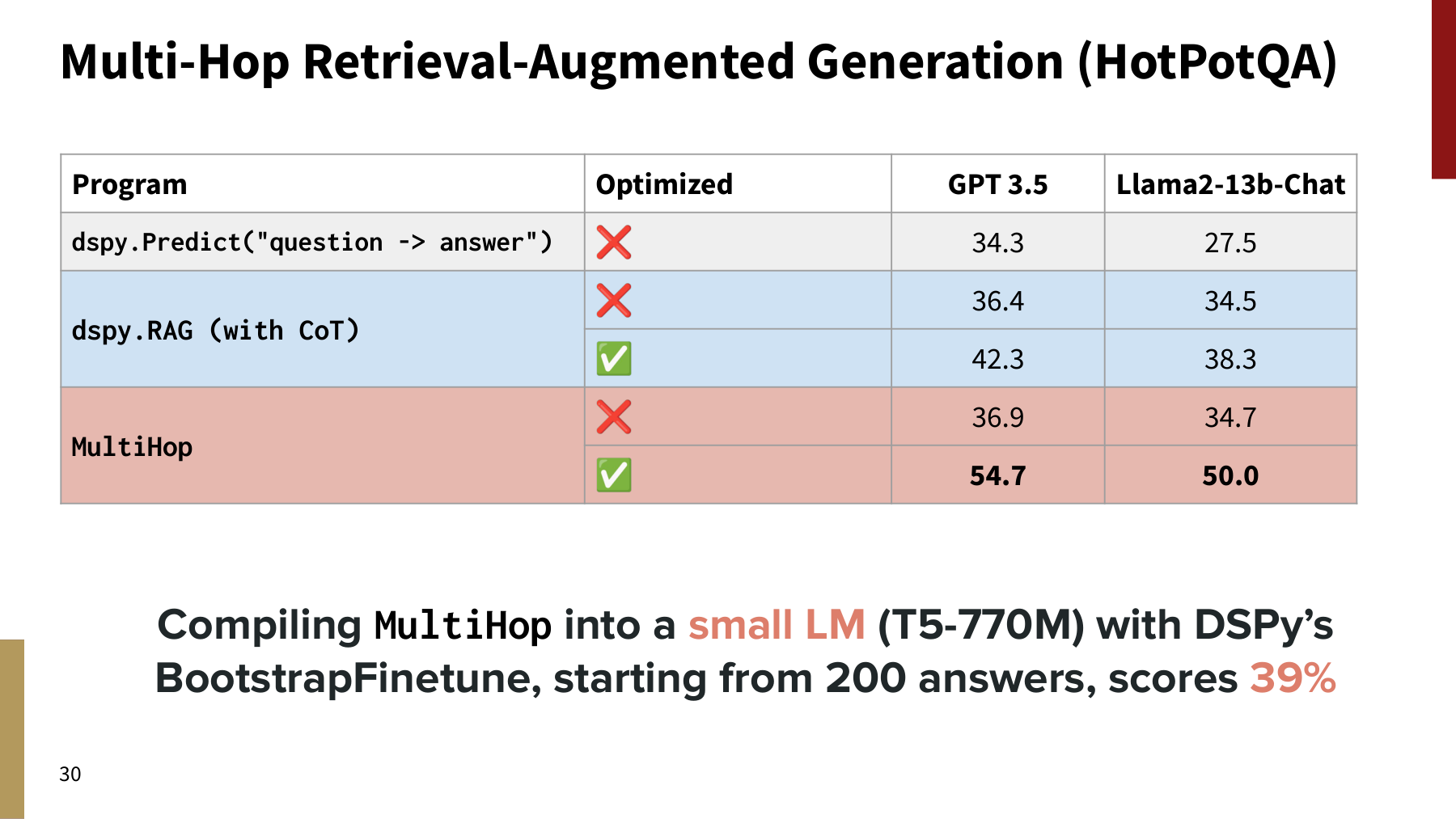
Omar Khattab’s DSPy lecture compares the same MultiHop program before and after optimization. With GPT-3.5, its score rises from 36.9 to 54.7. This is the lecture’s HotPotQA comparison. Other models and datasets require separate tests. The BootstrapFinetune results for the smaller T5-770M also use different models and training conditions and should be read separately. Lecture, p. 30
#Worked example 1. How can the agent retrieve the right memory and still fail?
Imagine 100 new problems. A retrieval counts as a hit if at least one returned experience contains evidence useful for solving that problem. Let r be the hit rate, u the probability of a correct answer given a hit, and v the probability of a correct answer given a miss. The model can still solve some problems on its own. Weight the two groups by their frequency to obtain the overall accuracy A. The counts below are illustrative.
Suppose the retriever hits on 80 problems and the model answers 60 of those correctly. Then r = 0.80 and u = 60/80 = 0.75. It also solves five of the 20 misses, giving v = 5/20 = 0.25.
That gives 65 correct answers. Raising the hit rate alone to 90% gives 70% accuracy if u and v stay fixed. Keeping the retrieved contexts identical and raising only u to 85% gives 73% accuracy. In a real system a new retriever can change which problems count as hits and how long their contexts are. Record retrieval hits and final correctness for each problem to diagnose a change.
Liu and colleagues isolated a further variable in Lost in the Middle. In multi-document question answering, moving the answer-bearing document from the beginning or end toward the middle reduced accuracy for several models. An analogous agent experiment could keep the retrieved experience and distractors fixed and vary only their order. That would test whether the agent uses evidence once it has been retrieved. The paper tested document QA and key–value retrieval. Reordering agent trajectories is the application proposed here. Liu et al., TACL 2024
#Part II, p. 22 — BetterTogether combines prompt optimization and fine-tuning
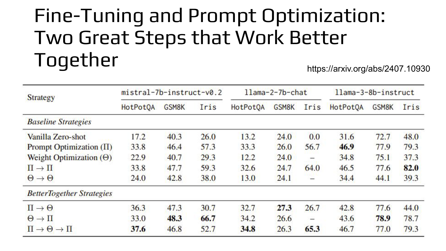
This slide reproduces Table 1 from Fine-Tuning and Prompt Optimization: Two Great Steps that Work Better Together by Soylu, Potts and Khattab (EMNLP 2024). The authors tested whether the final task score could guide optimization of a modular language-model pipeline without ground truth for intermediate steps or gradient information for every module. Paper
On the slide, Π denotes prompt optimization and Θ denotes weight optimization. Arrows give the order of optimization. Π → Θ → Π describes how to prepare the system: improve the prompt, fine-tune the weights, and optimize the prompt again for the new weights. These are training stages, not three prompts run in sequence at inference.
| Paper notation | Update order | Component changed |
|---|---|---|
| Π | Prompt optimization only | Instructions and examples in h |
| Θ | Fine-tuning only | Model weights θ |
| Π → Θ | Prompts → weights | First h, then θ |
| Θ → Π | Weights → prompts | First θ, then h |
| Π → Θ → Π | Prompts → weights → prompts | Search again for h under the new θ |
#Reading the original table
On HotPotQA with Mistral-7B-Instruct-v0.2, Π alone scores 33.8 and Π→Θ→Π scores 37.6, a gain of 3.8 percentage points. No sequence wins everywhere. On Iris with Llama-3-8B-Instruct, Π→Π scores 82.0 and Π→Θ→Π scores 79.3, a decline of 2.7 points.
A dash in the table marks an unreported condition with too few training examples. It does not mean a 0% failure rate. Changing the dataset or initial prompt can change which sequence wins. Soylu et al., Table 1
To isolate order more closely, compare rows with the same number of stages. In the Mistral-7B HotPotQA column, Π→Θ scores 36.3% and Θ→Π scores 33.0%, a 3.3-point difference. On GSM8K the same model scores 47.3% and 48.3%, reversing the ranking. Each number averages held-out accuracy over three seeds. In the HotPotQA program, two modules generate successive search queries and a third generates the answer. Even with a frozen retriever, changing the first query prompt can change the documents returned and the input to the second module. Starting with Π can thus change which successful traces are available for Θ to learn from. This gives a mechanism for an order effect. The scores alone cannot attribute a share of it to a specific module. Soylu et al., Table 1 and experimental setup
#What does the algorithm do?
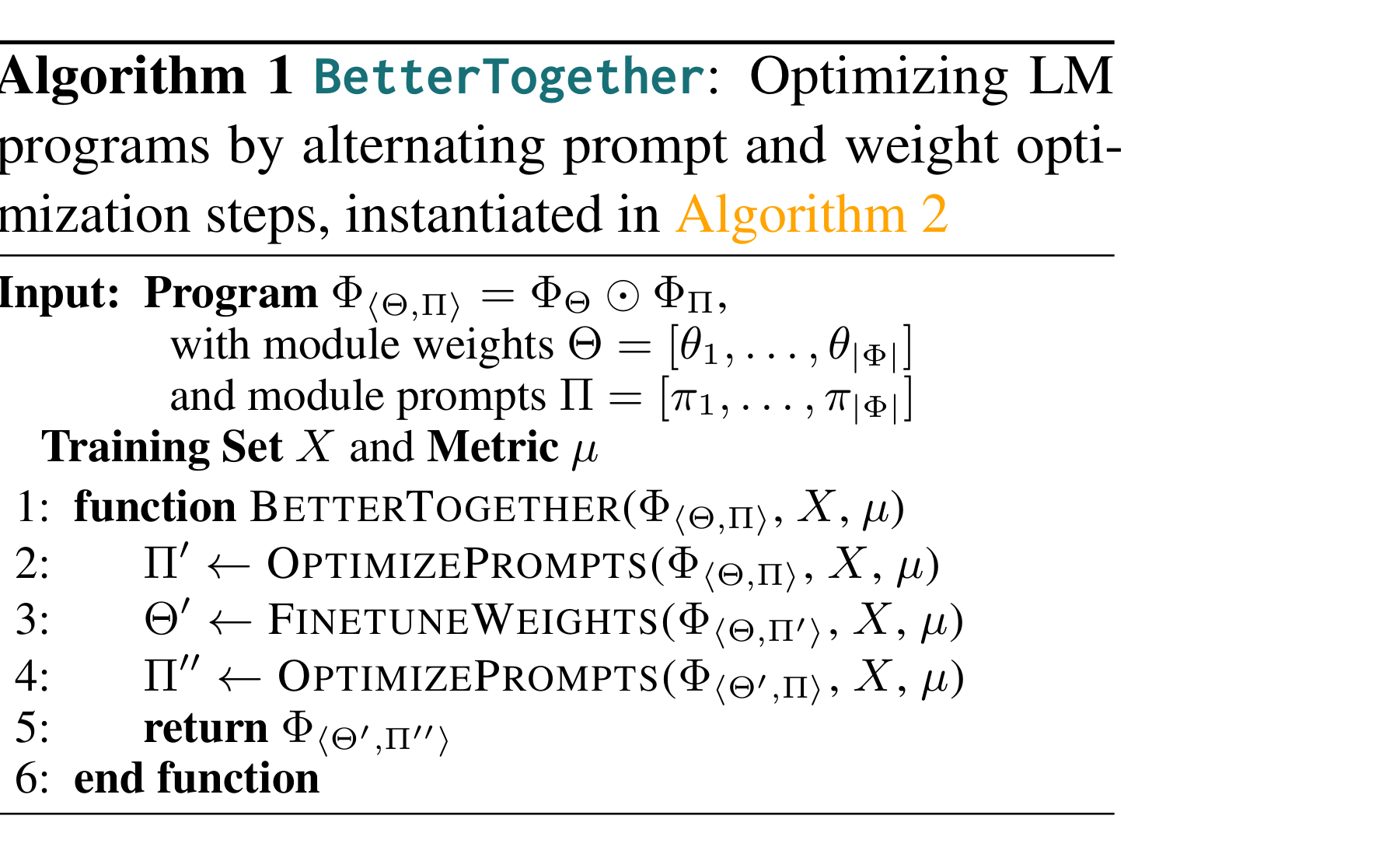
The meta-optimizer alternates between collecting good few-shot demonstrations for a prompt and training module weights on data synthesized from intermediate program trajectories. Each stage needs a measurable end-task quality metric. Running the three stages more often does not necessarily help. Measure performance on fresh evaluation data alongside model-call and training costs. BetterTogether, section 3
#Supplementary lecture — A final metric can guide module improvement
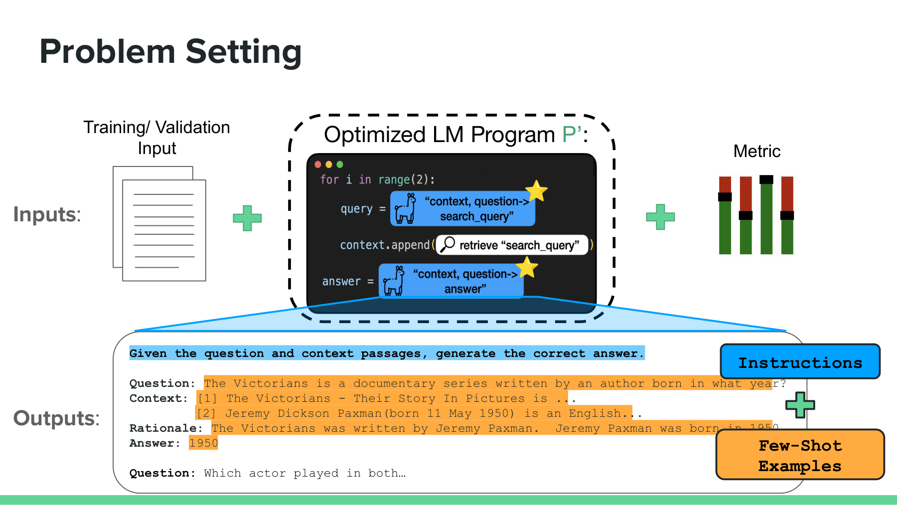
On page 35 of Khattab’s lecture, “Instructions” and “Few-Shot Examples” appear between the inputs and LM Program P′. The evaluator observes a metric for the final result. The query-generating module and the answer-generating module may each lack human-labeled targets. Candidate training examples can instead be drawn from actual program trajectories, after which candidate programs must be evaluated on the entire task. Lecture, p. 35
#Part II, p. 23 — Why weight updates and harness updates differ
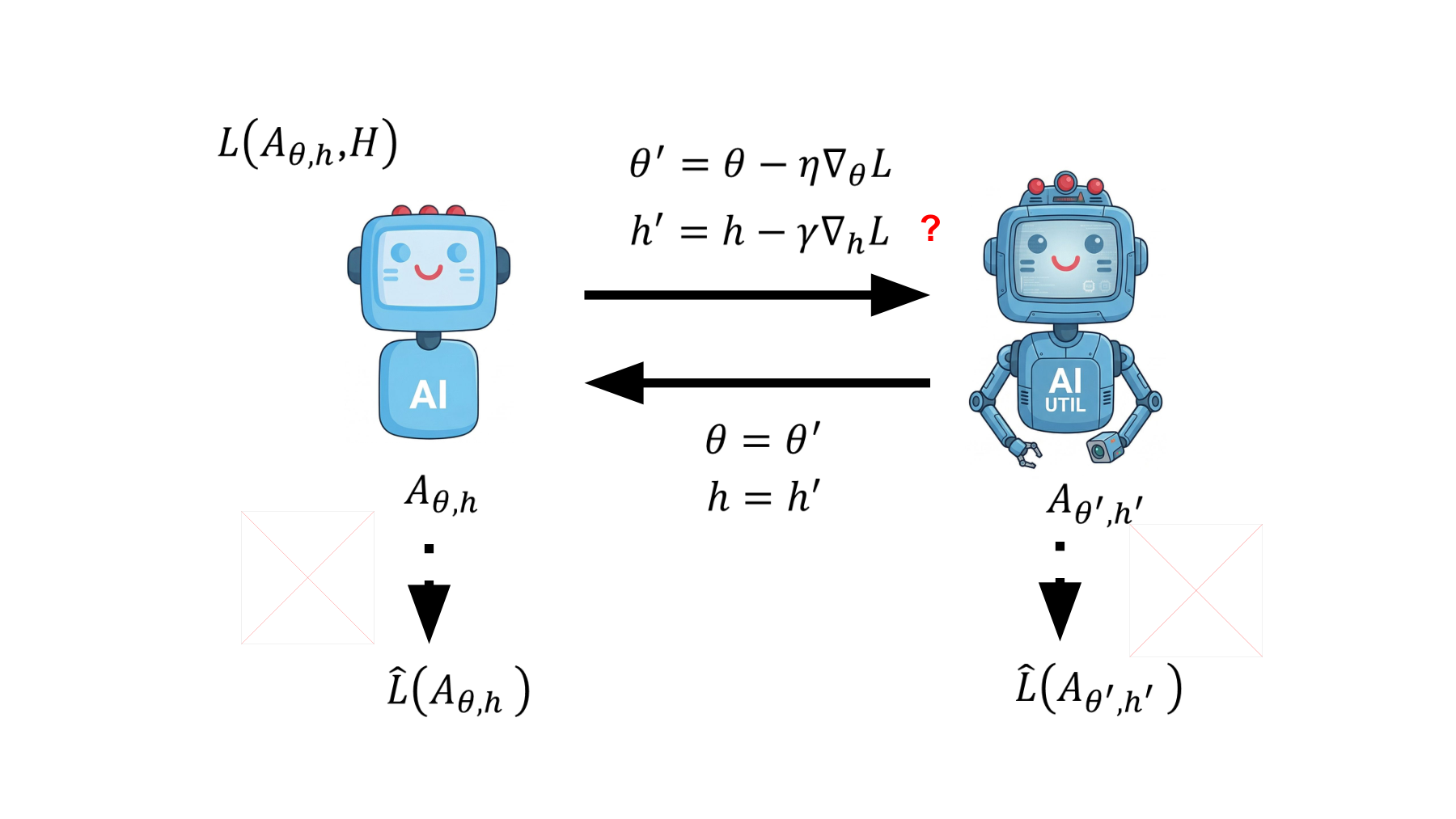
The slide’s first equation shows ordinary gradient descent. With continuous model parameters θ and a differentiable training loss L, the update is:
A question mark accompanies the next expression.
When h contains strings, JSON tool descriptions, a memory index, program branches, or code, treating it all as a continuous vector and applying the same gradient update is unjustified. A single word can cause a discontinuous change of execution path, and some components have no defined derivative.
A more general formulation is to generate, evaluate and select candidates.
Harness editing can be combined with weight training. The two may require different update rules. OPRO and GEPA propose and select prompt candidates, while DSPy and BetterTogether compose optimizers for individual modules.
#Supplementary lecture — What can the optimizer actually access?
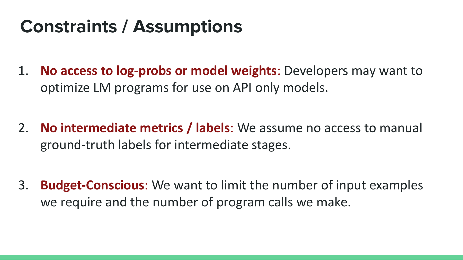
Page 36 of Khattab’s lecture lists three constraints. (1) An API-only model may expose neither log probabilities nor weights. (2) Human labels may be unavailable for intermediate modules. (3) Both experimental model calls and training data have budgets. Under these conditions, backpropagating through every component in one pass is not a general solution. Lecture, p. 36
When fine-tuning or LoRA is available, part of θ can be trained. To attribute any improvement, specify the trainable parameters θ, the fixed harness h, the data split, hyperparameters and model version.
#Which instruction deserves the credit, the query or the answer?
Follow MIPRO across pages 69–74 of Khattab’s lecture. Imagine that the first module writes queries and the second writes answers. Picking one instruction and one set of demonstrations for each module specifies one complete program. The slide sequence illustrates three trials scoring 75%, 50% and 80%. Each score belongs to the full combination. Moving the query instruction from the 80% trial into a different answer module could change the result. Khattab, lecture slides 69–74
MIPRO’s Bayesian optimizer uses the choices made in each trial and the score observed for the full program to propose another combination. At 54:13 in the Berkeley recording, Khattab illustrates the budget with 200 validation examples. A trial can sample 30, evaluate the selected combination and feed the observed score back into the surrogate model. The sampled examples affect that score. Berkeley lecture at 54:13
Slide 74 shows a return to the full validation set at regular intervals, which helps check whether a promising score came from unusually easy examples in a small batch. This gives a concrete answer to the question mark on slide 23. Even when a sentence has no numerical gradient, two complete programs can be run on the same problems and compared. Opsahl-Ong et al., Algorithm 1
#Part II, p. 24 — E-SPL runs system-prompt evolution alongside RL
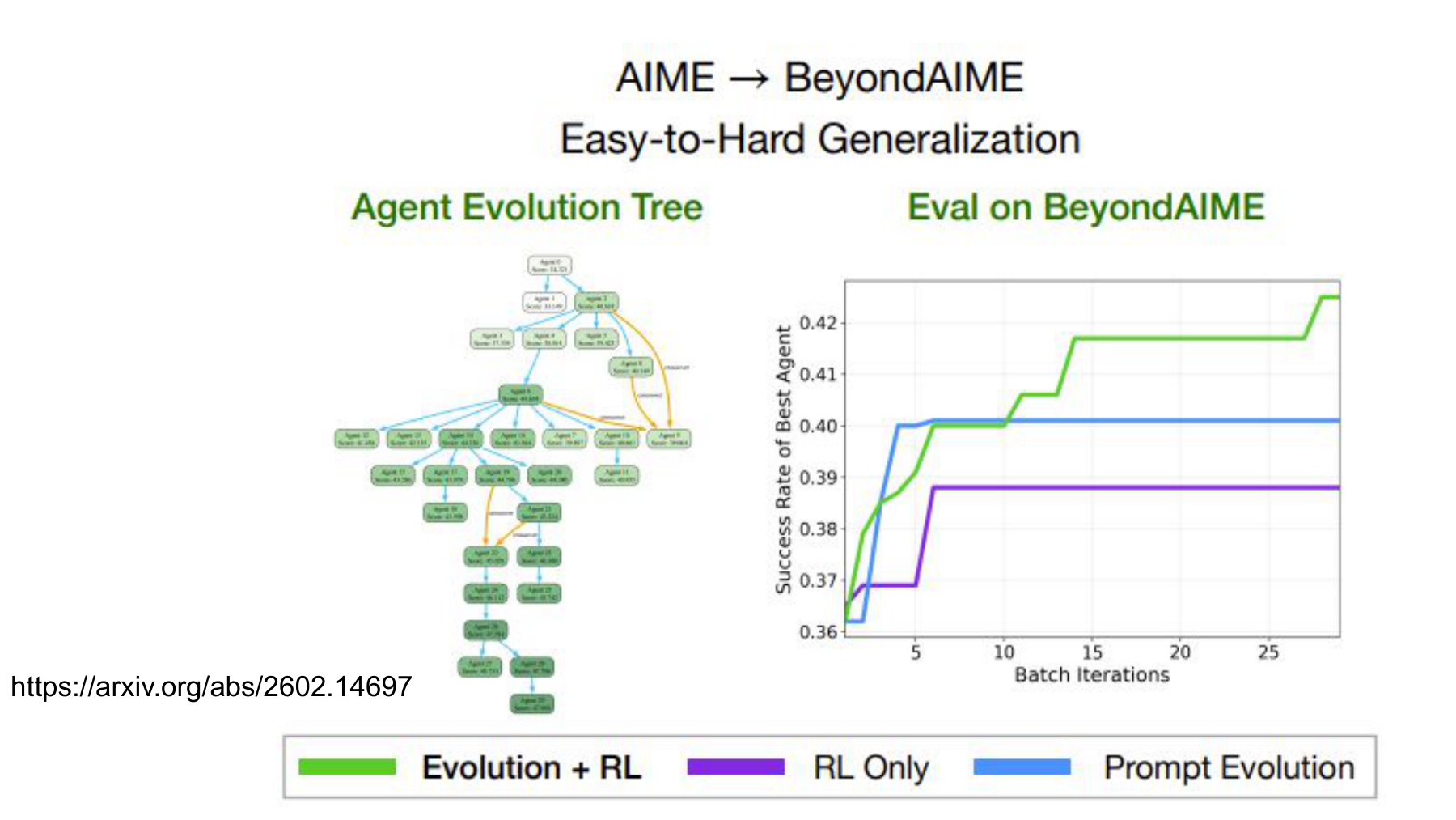
The NTU slide shows an agent evolution tree on the left and easy-to-hard generalization from AIME to BeyondAIME on the right. The source is the 2026 paper Evolutionary System Prompt Learning for Reinforcement Learning in LLMs. arXiv
Evolutionary System Prompt Learning (E-SPL) goes beyond replicating DGM. Inside a single RL training loop, it generates answer trajectories with different candidate system prompts and reuses the outcomes in two ways.
- Weight update: RL updates the model parameters θ using rewards for individual problems.
- Context update: Relative prompt scores and records of failures inform mutation and crossover, producing the next instructions.
Since both the prompt population and the model weights change, absolute scores across rounds need not be comparable. E-SPL ranks candidates that share the same problems and model within a round and combines these comparisons using a TrueSkill-style running assessment. E-SPL, section 3
Here μ is a candidate’s estimated mean skill and σ its uncertainty. The parameters λ and T control exploration and exploitation. A candidate can be explored for its uncertainty as well as for high mean performance. This expression illustrates the search model. The paper gives the choices for individual settings.
#Worked example 2. Why test a candidate with a lower mean rating?
Appendix B of E-SPL sets λ to 2. Suppose prompt A has a mean rating and standard deviation of (25, 1), while B has (23, 2.5). These are illustrative values on the TrueSkill rating scale. A rating of 25 does not imply 25% accuracy. A’s selection score is 25 + 2 × 1 = 27. B’s is 23 + 2 × 2.5 = 28. Set the temperature T in the paper’s selection equation to 1. For one draw from these two candidates, the probability of choosing B is
B has a lower mean rating and still gets a 73.1% chance of being tested. Testing an uncertain candidate provides evidence that can distinguish an early lucky result from a reproducible one. Being sampled does not automatically make B the parent of a new prompt. The algorithm runs the sampled candidates on the same problems under the current weights and mutates the candidate with the highest average reward in that round. Selection for a trial and winning that trial are different events. E-SPL, Algorithm 1 and section 3 · Appendix B
#What do the three curves compare?
The paper reports the following AIME-to-BeyondAIME success rates.
| Method | Success rate | Interpretation |
|---|---|---|
| RL only (GRPO) | 38.8% | Update weights with a fixed prompt |
| Prompt evolution | 40.0% | Evolve the prompt with fixed weights |
| Evolution + RL (E-SPL) | 45.1% | Combine prompt evolution and weight training |
E-SPL gains 6.3 percentage points over RL only and 5.1 points over prompt evolution. These are reported scores on the same dataset. Other models, tasks and budgets can yield different gains. A strong result on this test also needs verification on subsequent evaluation problems. Figure 7, DeepSeek-v3.1
#Why combine the two updates?
Prompts can express readable declarative knowledge such as solution strategies and cautions. Weight updates can change how the model executes those strategies through repeated experience. E-SPL proposes and tests the idea that this division of labor can help generalization. It does not establish that all procedural knowledge resides exclusively in weights or all declarative knowledge exclusively in prompts.
#Part II, p. 25 — The improvement goal itself can change
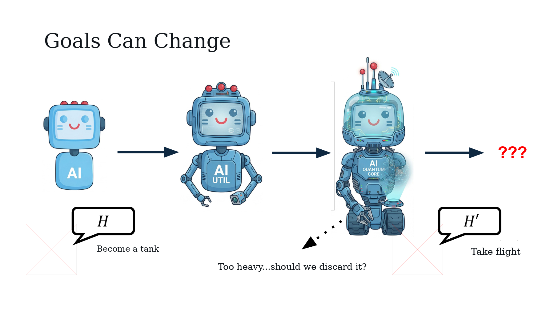
The final drawing is titled Goals Can Change. A robot acquires a heavy tank-like structure to become stronger. When the new goal is to fly, the added parts weigh it down. The analogy illustrates why an improvement under one objective needs another test under the next.
If the objective H varies with time, a single fixed score cannot determine whether a change counts as an improvement.
This notation illustrates objectives that depend on context. It does not imply that optimization finds a global optimum at every time step.
Consider a robot initially tasked with moving objects quickly. Aggressive path planning and high acceleration may help. When its objective becomes safe collaboration near a person, collision risk, approach speed, safe stopping and sensor latency become priority constraints. A candidate that violates them should be rejected even if it reports a high task success rate. A change of goal can alter the evaluation function, constraints and operating environment together.
#Worked example 3. When can the winner change with both models frozen?
Suppose two vision agents read labels and inspect surfaces for scratches. On fixed evaluation sets, A achieves 96% accuracy for labels and 60% for scratches. B achieves 82% and 90%, respectively. Assume each inspection is worth the same. Let w be the fraction of inspections that involve labels and 1 − w the fraction involving scratches. S is the expected accuracy across the workload, expressed in percent.
When labels account for 80% of work, A scores 88.8% and B scores 83.6%. At a 20% label share, A scores 67.2% and B scores 88.4%. Neither model was retrained. Solving 60 + 36w = 90 − 8w gives w = 30/44 ≈ 0.682. A leads when labels make up more than about 68.2% of inspections.
Now keep the same 80% label workload and change only the price of an error. Charge one loss unit for each wrong label decision and four for each wrong scratch inspection, with a uniform cost within each task. A’s expected loss per inspection is 0.8 × 0.04 + 4 × 0.2 × 0.40 = 0.352 units. B’s is 0.8 × 0.18 + 4 × 0.2 × 0.10 = 0.224 units. A wins on accuracy, but B incurs less loss. If missed defects and false alarms have different costs within the scratch task, aggregate accuracy cannot determine this choice. The calculation would need the error rates for each type. Episode 19 separately examines forgetting by retesting performance on the same earlier task.
#Keeping the best candidates when the current goal changes
A system that updates both θ and h should preserve their versions and evaluation conditions separately. Obsolete memories or tool calls should be removable from the active system, while its earlier behavior and safety regression tests remain reproducible. Without a record of past objectives, it is difficult to verify a claim of self-improvement.
#Five slides together: what changes, and what is evaluated?
| Approach | Optimization target | Improvement signal | Evaluation detail |
|---|---|---|---|
| ExpRAG + fine-tuning | Retrieved experience and model weights | Past trajectories, correct answers, rewards and training loss | Isolate the effects of retrieval and weight changes |
| BetterTogether | Module prompts Π and weights Θ | Final metric and intermediate trajectories | Specify the sequence, dataset and experimental budget |
| E-SPL | System-prompt population and RL policy | Within-round relative performance and reward | Keep absolute scores from different model versions separate |
| Goal change | Objective H and selection criteria | New evaluation metrics and constraints | Reevaluate past optima under the current goal |
Across these five slides, improvement is an experimental claim: specify the component changed and the objective it was changed to serve. Episode 19 starts on page 26 of Part II with test-time training (TTT) and forgetting.
Check the calculations
Turn off the uncertainty bonus in example 2 by setting λ = 0. The remaining scores are the means, 25 and 23, so the chance of selecting B falls to 1/(1 + e²) ≈ 11.9%. In example 3, set w = 0.5. A scores 78% and B scores 86%. Both scores use unchanged per-task accuracies, so this gap measures the workload mix rather than a loss of prior skill.
#Further reading
| Source | Material used here |
|---|---|
| NTU Part II, pp. 21–25 · Lecture video | Five primary lecture slides |
| ExpRAG, EMNLP 2026 | Retrieving experience and learning to use it |
| BetterTogether, EMNLP 2024 · arXiv v2 | Alternating prompt and weight optimization, Table 1 and Algorithm 1 |
| Omar Khattab, Compound AI Systems & DSPy | Supplementary lecture slides 30, 35 and 36 |
| DSPy BetterTogether documentation | Optimizer concepts and conditions for invoking them |
| E-SPL, 2026 · Official implementation | Joint prompt evolution and RL, and generalization from easier to harder problems |
The numerical results from the papers apply to their experimental settings. Page 25 of Part II is an unofficial edit with English labels. Consult the original for its wording.