Learning begins with changing an answer. It can also change which answers a model tries more often and which problems it chooses to solve.
Part 8 — To minimize entropy, find the missing gradient showed that differentiating a loss with the sample fixed misses the change in the sampling distribution. Here we ask which paths the missing term favors. After a speech recognition experiment, we widen the question. What changes when AI supplies the training inputs as well as the scores for the outputs?
Video timestamps by slide
| Slide | Video segment and topic | Related concept |
|---|---|---|
| 41 | 43:24–44:07 — Making low-entropy paths more likely | The missing logarithm, probability tree and baseline conditions |
| 42 | 44:07–44:51 — Speech recognition error rates on three corpora | EM-tok versus EM-tok-b, comparison conditions and error reductions |
| 43 | 44:51–44:55 — End of the mathematical section | Correct gradients and actual accuracy |
| 44 | 44:55–45:19 — People still select inputs for an AI evaluator | Evaluator, reward model and policy |
| 45 | 45:19–45:39 — Delegating input generation to AI | Training input distributions and generation and filtering in Self-Instruct |
#Slide 41 — Changing a path and choosing a path
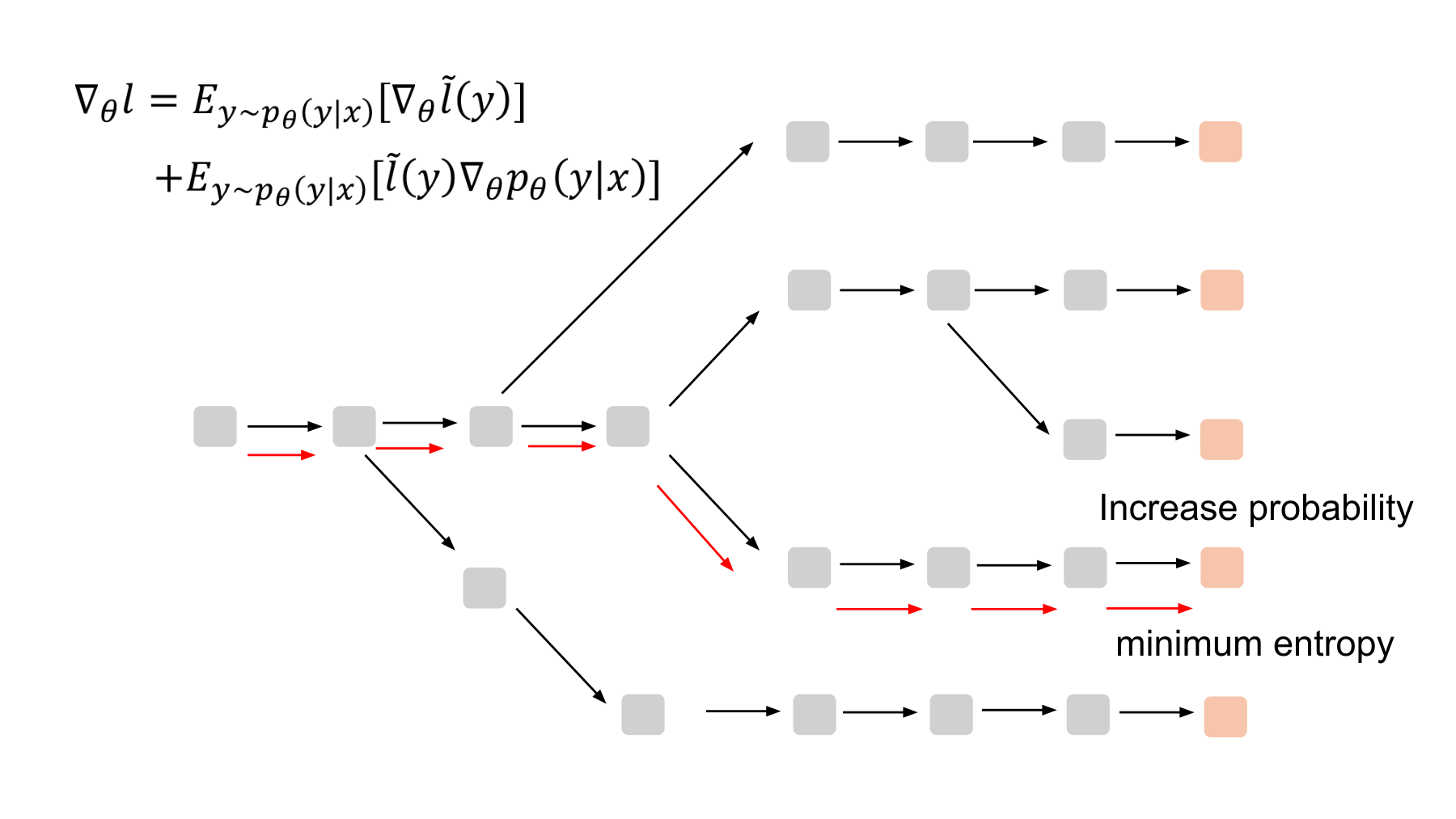
In the video · 43:24–44:07. The lecturer distinguishes two effects. The first reduces entropy along a path that has already been sampled. The second raises the probability of sampling low-entropy paths. The two work together.
A path is one generated sequence from its first token to its last. The figure’s “minimum entropy” label illustrates the intuition. Training need not enumerate every possible sentence and identify a single global minimum.
#Reading the two terms again
Fix the input x. Let Y be the sentence generated by the model and pθ its distribution. Define gθ as the sum of next-token entropies at the prefixes visited.
With appropriate sampling and termination conditions, the expectation of this quantity equals sequence entropy. Our finite example always generates two tokens, so interchanging the sum and derivative presents no difficulty.
Differentiating the expectation gives two terms. We reorder equation (8f) of the paper for readability.
A changes the entropy of the next-token distributions with the sampled prefixes fixed. B also adjusts the probability of generating the path. Neural networks share parameters, so the terms need not act on disjoint parameters. The split identifies different ways the calculation depends on those parameters. Paper, PDF p. 3, equations (8)–(9)
A correction to the notation. The second term in the image omits log. Inside an expectation we need the log-probability gradient. The log-derivative identity makes the following two expressions equal.
The sum on the left has no separate probability weight. The expectation on the right already includes one. Dropping log when converting to an expectation introduces an extra factor of the probability. Equation (8f) also uses the log-probability gradient.
#Checking the direction with a small probability tree
Consider a two-token tree. The first token is A or B. The next-token probabilities are fixed at 0.9 and 0.1 after A, and 0.6 and 0.4 after B. Only the probability p of the first branch varies, through its logit θ.
Binary entropy is measured in nats because we use natural logarithms.
| First branch | Next-token distribution | Next-step entropy |
|---|---|---|
| A | 0.9, 0.1 | h(0.9) ≈ 0.325083 |
| B | 0.6, 0.4 | h(0.6) ≈ 0.673012 |
The next token is less uncertain after A. The total two-token entropy combines the uncertainty of the first branch with the conditional entropies of the branches below it.
Start at θ=0 and p=0.5. The first-branch entropy h(p) has zero gradient there. The downstream distributions are fixed, so the fixed-sample term A alone cannot change the first branch probability. Term B, however, captures the entropy difference between the two branches.
Gradient descent subtracts the gradient, so a negative gradient increases θ. One update at a learning rate of 0.1 gives
The probability of the less uncertain A branch rises from 0.5 to approximately 0.5022. Before the update the four sentence probabilities are 0.45, 0.05, 0.30 and 0.20. The full entropy falls from about 1.192195 to 1.191428 nats.
This checks the direction of the gradient and the probability change. The example does not tell us whether A is the right answer. Low entropy and correctness are separate properties, so the calculation cannot establish an accuracy gain.
#Further reading A — A baseline makes relative path costs visible
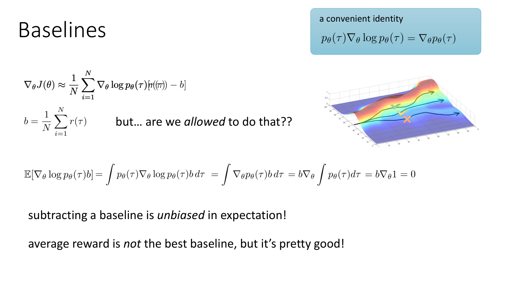
The Berkeley slide explains why we subtract a baseline in a policy gradient. Here we use entropy cost minimization instead of reward maximization. An update favors paths with below-average cost. Berkeley Policy Gradients, PDF p. 17
For a fixed baseline b(x) independent of the current sample Y, we can write
This is not an arbitrary change to the score. The expected gradient contributed by the baseline is zero because the probabilities sum to one.
In the example with p=0.5, fix the baseline for this update to the current expected cost of 1.192195.
| Path | Sum g of path token entropies | g−b | Interpretation |
|---|---|---|---|
| Begins with A | 1.018230 | −0.173964 | Below-average cost |
| Begins with B | 1.366159 | +0.173964 | Above-average cost |
The sign can be confusing if you are used to reward advantages in policy gradients. Here g−b is a cost difference. With reward r=−g, the corresponding reward advantage has the opposite sign.
Baseline independence. The slide also illustrates using a batch mean. A mean that includes the current sample is dependent on that sample. With G independent, identically distributed samples, subtracting a mean that includes each sample without further normalization scales the expected policy gradient term by (G−1)/G. At G=2 the expected term is halved.
To reduce policy gradient variance, the paper uses a leave-one-out baseline that excludes the sample itself. Independent sampling then also avoids the issue with the inclusive mean.
With independent samples, bᵢ computed from the other samples is independent of the current yᵢ, preserving the expected policy gradient. The expression is undefined at G=1, and the paper uses no baseline in that case. Paper, PDF p. 4, equations (13)–(16)
Automatic differentiation requires a stop-gradient on the cost difference. Using sequence sums without length normalization gives the following surrogate loss.
Both terms come from differentiating a single expectation. An implementation may rescale one term for stability, but the resulting direction no longer equals the exact gradient of the original entropy in general. The paper also adds token-count normalization and a beam-search extension, so distinguish the basic identity from the conditions of the training procedure. Paper §3.5
#Slide 42 — First ask what the results table compares
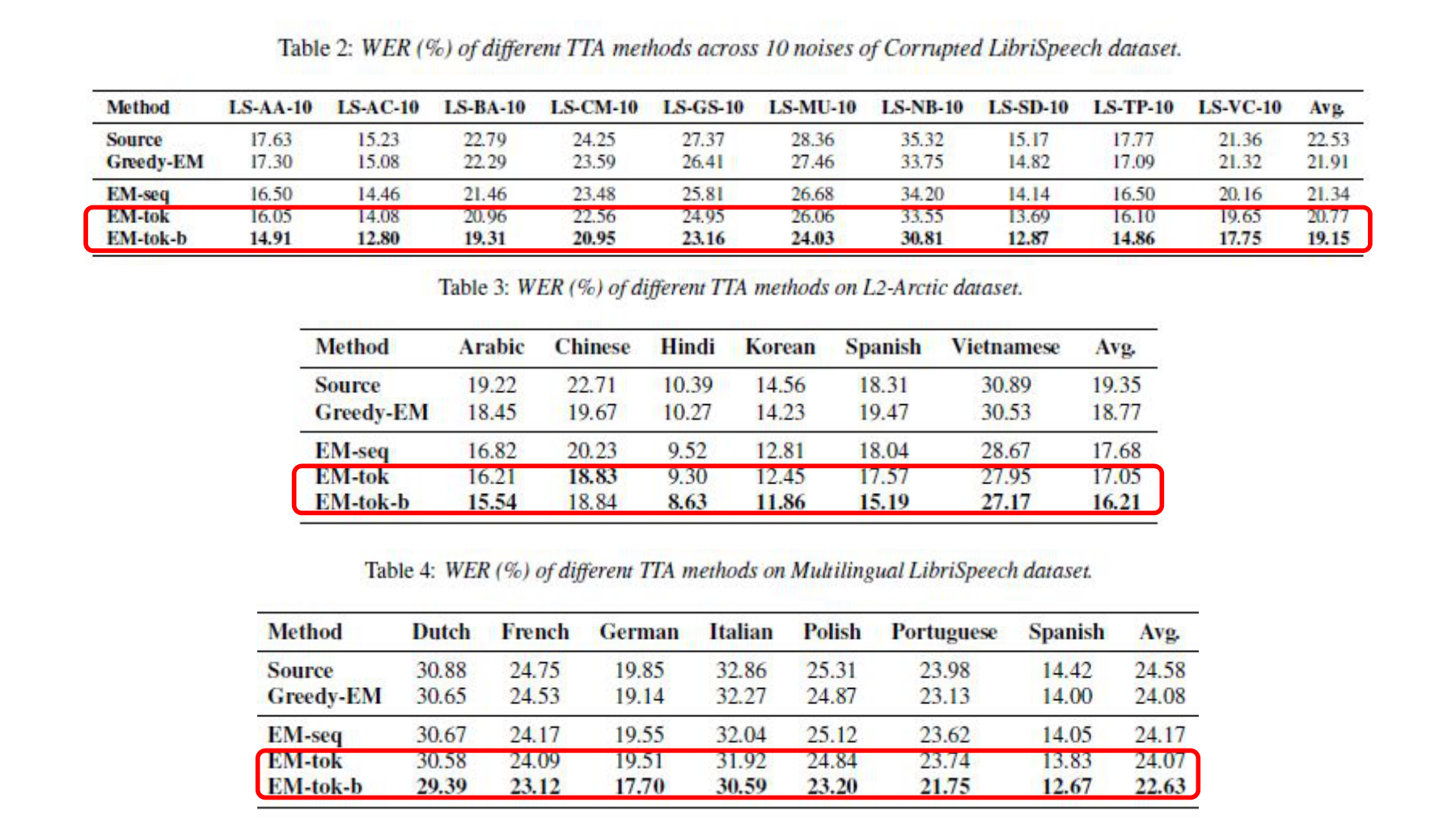
In the video · 44:07–44:51. The lecturer compares speech recognition error rates on three corpora and explains that lower is better. At about 44:13 he explicitly says that the experiment concerns speech recognition rather than general language model tasks.
#What differs between the methods? Candidate generation
The two rows outlined in red are EM-tok and EM-tok-b. To interpret them, first look at how each method produces candidates for training.
EM-tok and EM-tok-b both include both token entropy gradient terms. The b in EM-tok-b stands for beam search. The difference between the rows therefore does not isolate the effect of adding a gradient correction. Paper, PDF p. 5, §4.2
| Method | Candidate transcripts used for adaptation | Optimization |
|---|---|---|
| Source | No adaptation | Original model’s error rate |
| Greedy-EM | One greedy-decoded transcript | Optimizes only token entropy on a fixed transcript |
| EM-seq | G random samples | Policy gradient of the sequence-level estimator |
| EM-tok | G random samples | Direct token entropy term plus policy gradient |
| EM-tok-b | Top G beam candidates | Practical extension applying EM-tok to beam-search candidates |
Having only a policy gradient does not by itself make EM-seq incomplete. For the sequence-level estimator −log pθ(Y), a separate derivation gives a zero expectation for the direct term. Changing the estimator changes which terms are needed. Paper, PDF p. 4, equations (10)–(12)
Beam search also differs from random sampling under the model distribution. Section 3.5.2 explicitly notes the resulting bias. Better empirical performance and an unbiased gradient under the original distribution are distinct claims.
#WER measures word errors
Word error rate (WER) counts the substitutions, deletions and insertions needed to align a transcript with the reference.
S counts substitutions, D deletions, I insertions and N words in the reference. If a 100-word reference yields 10 substitutions, five deletions and three insertions, WER is 18%. With enough insertions it can exceed 100%, so it is not generally the complement of accuracy.
The following numbers come directly from the Avg. columns in the original tables. They are not a pooled WER recomputed from all reference words across corpora. Paper, PDF p. 6, Tables 2–4
| Method | Noisy LS-C | Non-native English L2-Arctic | Multilingual MLS |
|---|---|---|---|
| Source | 22.53% | 19.35% | 24.58% |
| Greedy-EM | 21.91% | 18.77% | 24.08% |
| EM-seq | 21.34% | 17.68% | 24.17% |
| EM-tok | 20.77% | 17.05% | 24.07% |
| EM-tok-b | 19.15% | 16.21% | 22.63% |
LS-C contains noisy English speech, L2-Arctic contains English speech from speakers with various first languages, and MLS contains speech in multiple languages. In particular, L2-Korean denotes English spoken by native Korean speakers. Paper §4.1
The differences when moving from EM-tok to EM-tok-b are shown below. This is the candidate generation comparison described above.
| Corpus | Absolute WER reduction | Relative error reduction |
|---|---|---|
| LS-C | 1.62 percentage points | About 7.80% |
| L2-Arctic | 0.84 percentage points | About 4.93% |
| MLS | 1.44 percentage points | About 5.98% |
For LS-C, the two calculations are
Calling this a “7.80 percentage point improvement” would use the wrong units. The changes are calculated from the rounded WERs reported in the paper.
#Experimental conditions
The base model is Whisper-base. For each speech input, EM-seq, EM-tok and EM-tok-b perform ten adaptation steps with G=16 candidates per step. AdamW uses a learning rate of 0.001 and updates only the LayerNorm parameters in the encoder and decoder. Each step regenerates candidates with the updated model. Greedy decoding with the adapted model produces the final prediction. The model parameters are reset after each input. Paper §4.2–4.3
This is test-time adaptation with a reset for each input. The reported changes therefore do not accumulate as permanent self-improvement across inputs. The paper says it selected hyperparameters on a separate CommonVoice subset and used them across the target corpora.
#An ablation isolates the gradient terms
The term-by-term ablation is in Figure 2 of §5.1, separate from the two highlighted rows in Tables 2–4. It compares three methods.
- ENT-tok: Direct token entropy term only.
- PG-tok: Policy gradient term for token-level cost only.
- EM-tok: Both terms.
For noisy speech, English from native Spanish speakers, and Polish speech, the study varies G over 1, 4, 16 and 64. The paper reports that combining both terms generally performs well with multiple samples. At G=1 the leave-one-out baseline is unavailable and the policy gradient term can become unstable. Paper, PDF pp. 6–7, §5.1 and Figure 2
A mathematically necessary term does not guarantee better results at every sample count and learning rate. Estimator variance, sample generation, normalization and optimization all influence the actual update.
#Further reading B — Searching a model versus changing it
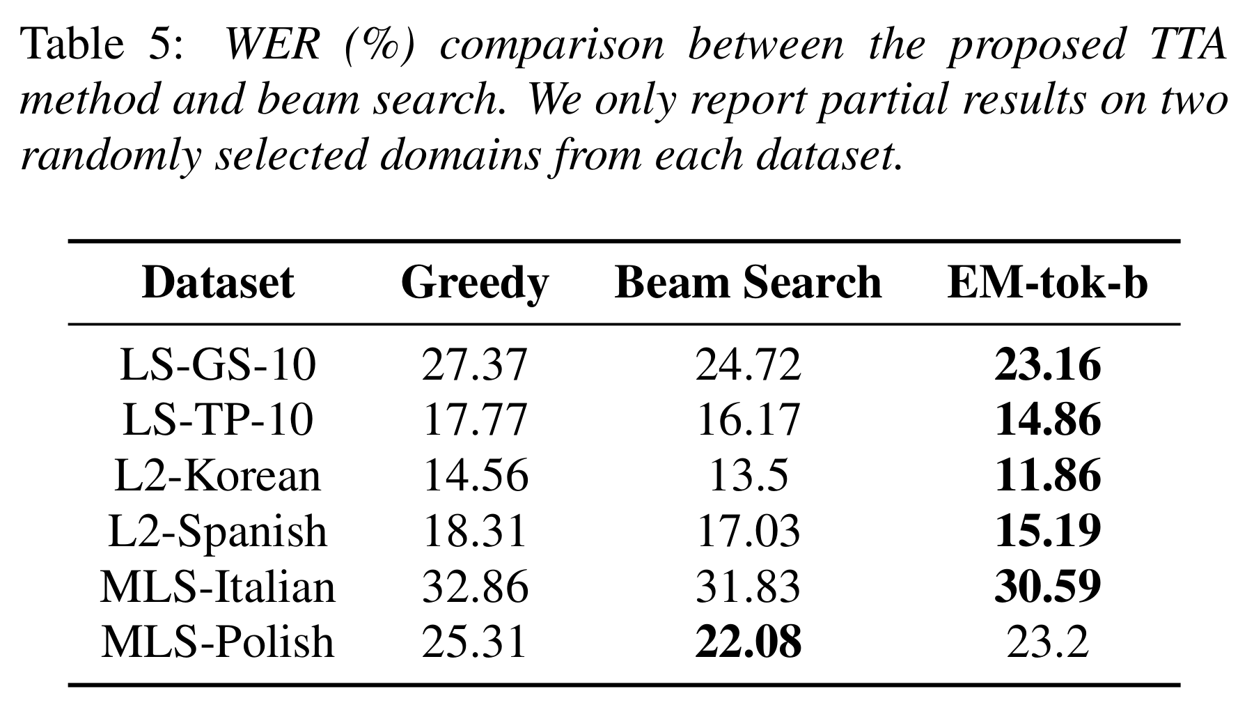
Table 5 compares beam search with fixed parameters against adaptation with EM-tok-b. The beam size is 16. The table reports two selected conditions per corpus, covering only part of the experiments. Paper, PDF p. 7, §5.2 and Table 5
| Example condition | Greedy | Beam search only | EM-tok-b adaptation |
|---|---|---|---|
| L2-Korean | 14.56% | 13.50% | 11.86% |
| MLS-Polish | 25.31% | 22.08% | 23.20% |
Adaptation gives lower error for English spoken by native Korean speakers. For Polish, beam search alone gives 22.08%, lower than 23.20% for EM-tok-b. The table thus includes a case where a decoding strategy without adaptation performs better.
There are two choices here. Decoding changes which output a search finds in a given model, and adaptation changes the model distribution itself. Evaluating a method that uses both calls for comparisons that separate their effects.
#Slide 43 — Three questions after the math

In the video · 44:51–44:55. This slide marks the end of the derivation. It introduces no new algorithm or experimental result.
Three questions summarize the preceding calculations.
| Question | What to check |
|---|---|
| Is my gradient the gradient of the objective? | Sampling distribution, direct and policy gradient terms, baseline independence |
| Does the adaptation procedure meet those conditions? | Beam-search bias, length normalization, sample count and update procedure |
| Does lowering the objective improve the capability I want? | Separate measures such as accuracy or WER, comparison conditions, per-input resets |
These distinctions also apply to AI evaluation. Even if AI supplies scores in place of a human-defined mathematical cost such as entropy, we still need to decide which score to optimize and how to evaluate the result. Slide 44 points to an earlier choice. Who selects the training problems?
#Slide 44 — If AI supplies the training signal, who selects the inputs?
Slides 41 and 42 examined how to calculate an entropy-reducing gradient. The lecture now returns to a broader question. Even if a model can evaluate its outputs and learn from them, who decides what problems it gets to solve?
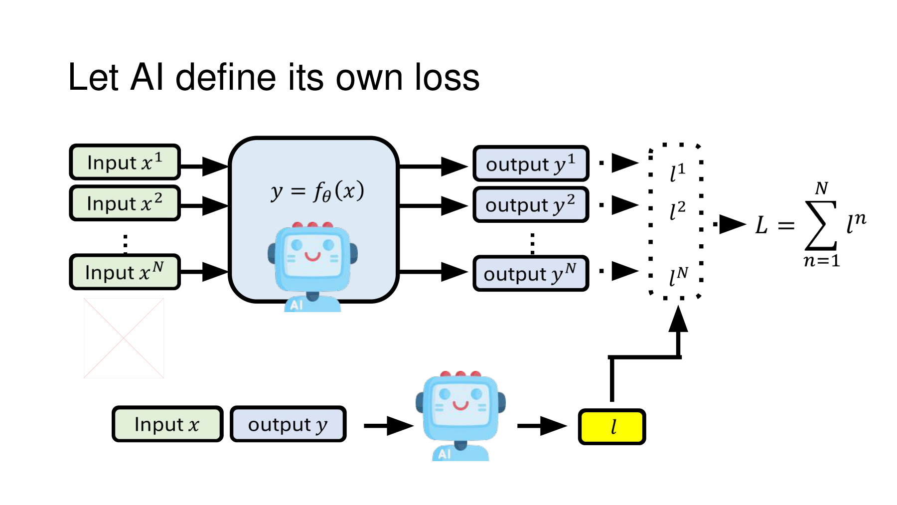
At 44:55, the lecturer revisits the idea of AI determining its own loss and training itself. He points out a job people still do: finding inputs and feeding them to the model. In slide 44 an evaluator AI already exists, but the list of inputs at the top still comes from outside.
The AI at the bottom assigns a loss to each input-output pair. The first point is that AI supplies an evaluation signal for learning. The diagram does not imply that AI invented a differentiable loss function or optimization algorithm. We still need an explicit link between scoring an answer and updating parameters.
#Further reading C — How does an evaluator’s score reach the policy?
Lee et al.’s ICML 2024 paper compares reinforcement learning from AI feedback (RLAIF) with RLHF, which uses human preferences. In RLAIF, AI evaluates response preferences. Those data train a reward model, and its scores improve the policy. The paper also presents direct-RLAIF, in which the evaluator supplies scores directly. Paper §2 and Figure 2
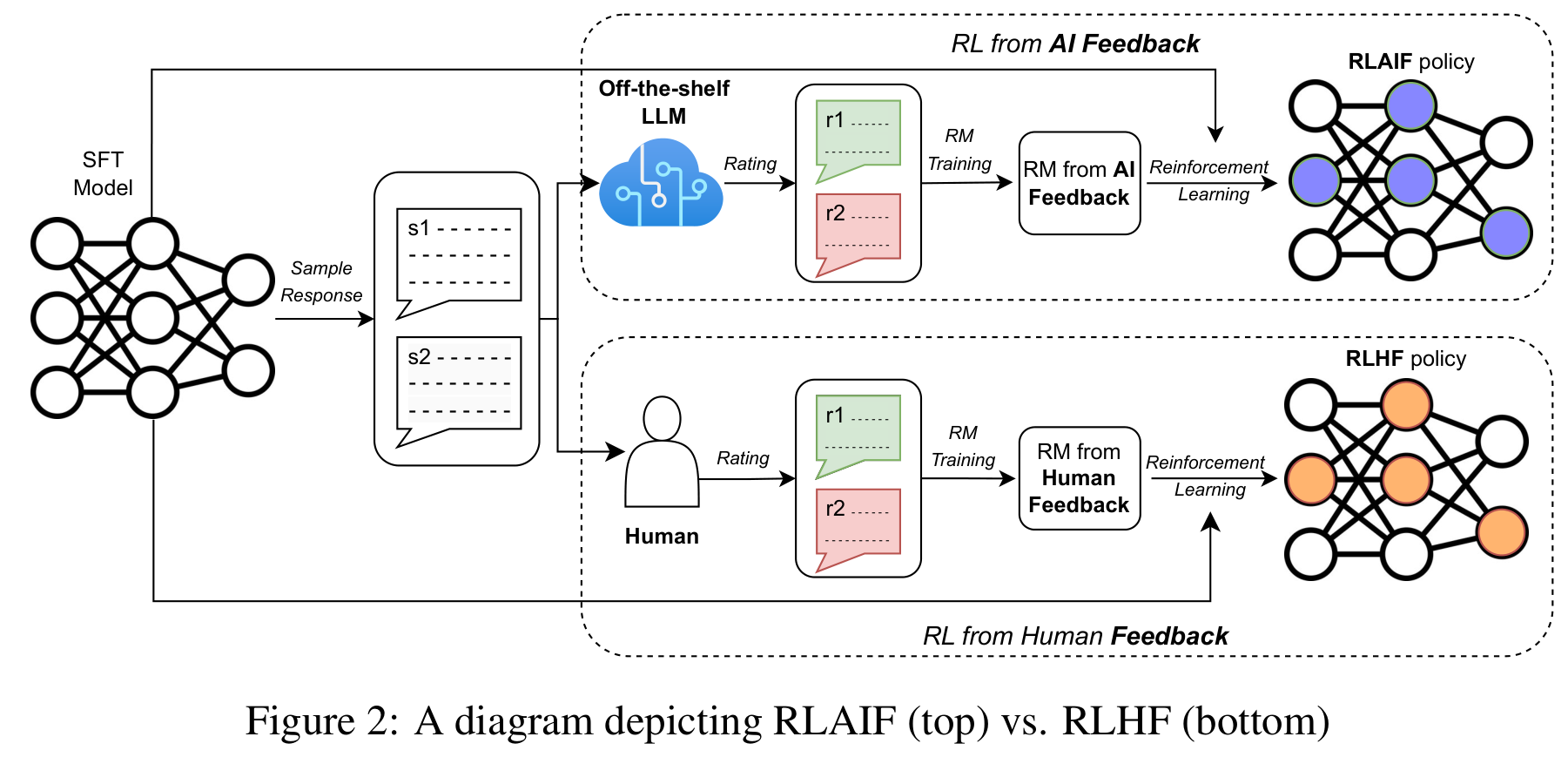
Three symbols make the roles easier to follow. Let be the input, the policy that generates an answer, and the evaluation function that scores it. Consider a simple setup that separates these roles.
Define rewards so that larger is better and losses so that smaller is better. The simplest relationship expressing one score from these two perspectives is
Calling backward() directly on the number returned by the evaluator generally does not train the answering policy. The sentence was generated by sampling discrete tokens. A policy gradient propagates the evaluation by specifying which answers should become more probable.
For example, during a single policy update we can hold the evaluator, the sampled inputs and the sampled responses fixed and differentiate this surrogate loss.
Here stops backpropagation and is a baseline score for the same input. If the current answer scores above baseline, gradient descent increases its log probability. A below-baseline score does the opposite. The sign is opposite to the entropy-cost example because here we favor higher rewards.
This explains why we distinguish the evaluator parameters from the policy parameters . The evaluation criterion is held fixed while the answering policy learns. Even if both roles start from the same checkpoint, the evaluator is not thereby updated in the same computation graph. Training the evaluator itself requires a separate training criterion.
Returning to slide 44, even an excellent evaluator can give a model practice only in single-digit addition if all its inputs are single-digit additions. The evaluator determines which answers are preferred. Input selection determines what the model gets a chance to learn.
#Slide 45 — Generating problems changes the training distribution
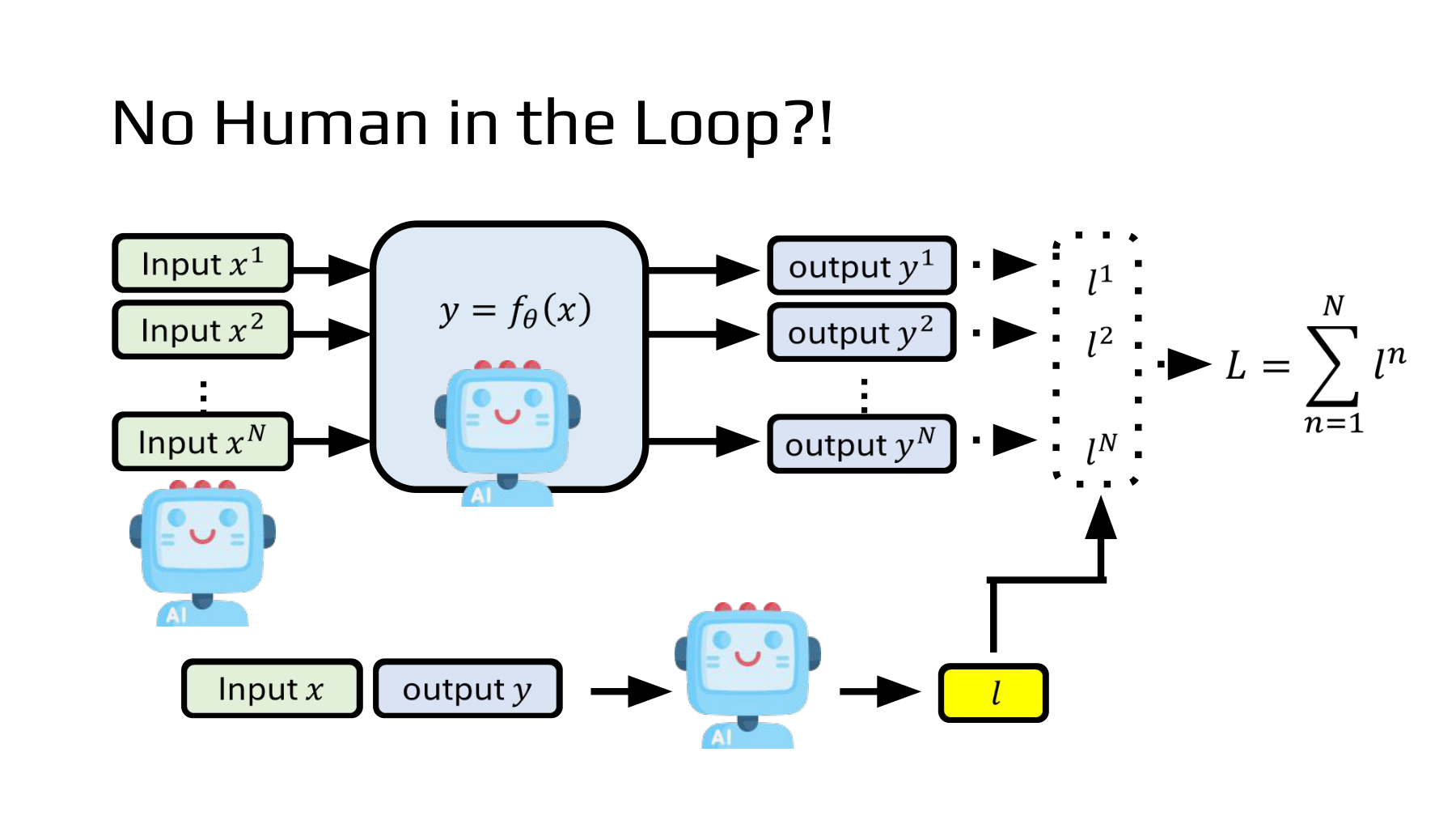
At 45:19 the lecturer asks whether a model could also find its inputs. It would find an input, produce an output, evaluate it and learn from it. Slide 45 adds an AI next to the input list. Its title, “No Human in the Loop?!”, asks how far this automation can go.
Writing the idea mathematically makes the input distribution explicit. Let be the input generator’s distribution. Holding that generator and the evaluator fixed for one policy improvement step gives a possible objective.
The objective separates input generation, answer generation and evaluation. One model can fill all three roles, but that does not require differentiating all parameters jointly through one loss. Each stage must specify which roles stay fixed and which parameters it updates.
Pay particular attention to . An input generator that frequently makes easy problems makes them more prevalent. Repeating a topic or a phrasing concentrates practice there. Even with the same evaluator and answering policy, a change in input distribution changes what the optimized average score represents.
Suppose a model was evaluated half on addition and half on multistep calculations. If its generator begins producing addition 90% of the time, mean training reward may rise. That alone tells us little about multistep calculation. We must check the mix of evaluation problems to identify which capabilities improved.
#Further reading D — Self-Instruct filters the generated data
Self-Instruct is a concrete example. Figure 2 of the ACL 2023 paper starts with 175 human-written seed tasks, generates instructions, inputs and outputs, filters low-quality or similar results, and adds the survivors to a task pool. Self-Instruct §2, Figure 2
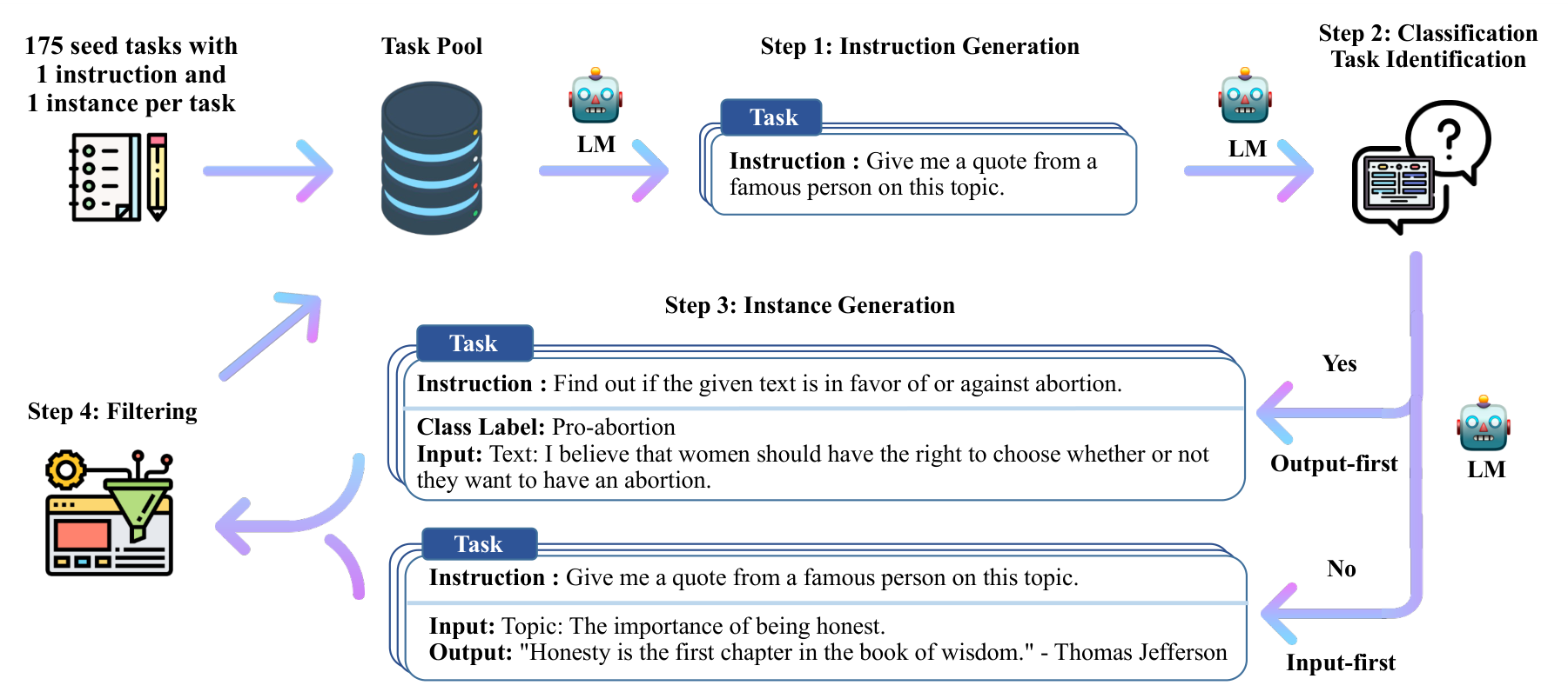
The filtering at the left matters as much as generation at the right. A model-generated item is not automatically accepted. After removing duplicates and format problems, among other issues, the paper uses the remaining data for supervised fine-tuning (SFT) of the original model. Paper §2.2–2.3, PDF pp. 3–4
In conventional notation, let combine the instruction and input, and let be the dataset fixed after generation and filtering. The negative log-likelihood for the target output tokens is
Here the generated output is a fixed training target. Earlier, policy gradients used scores on sampled answers to change their probabilities. This loss increases the probabilities of previously collected target outputs. Using self-generated data does not make both procedures reinforcement learning.
The 175 human-written seed tasks and the filters also matter when interpreting human involvement. A loop that needs no human to label every iteration can still rely on people for its starting point, selection criteria and performance assessment.
#What would we compare in an experiment?
Alongside the volume of generated data, record three quantities when turning slide 45 into a small experiment.
- Fixed held-out set. Measure performance before and after on the same problems, excluded from generation and training. Record mean training reward separately from accuracy on this fixed set.
- Input composition. Track counts by topic and difficulty, along with the duplicate rate. Check whether growth disproportionately favors one task type.
- Agreement between the score and actual success. Check a sample against an independent criterion such as code execution or arithmetic verification. This can reveal a rising evaluation score alongside a flat success rate.
These comparisons distinguish a generator making more problems, a model receiving higher scores from its evaluator, and a model solving new problems more successfully. Slide 45 asks under what conditions all three changes coincide.
Part 10 — Can a model keep getting smarter on problems it creates itself? examines the proposer, solver and verifier and why self-play needs external information.
#Read alongside the original
| Resource | Where to look | Connection |
|---|---|---|
| NTU Self-Improving lecture, first half | 43:24–45:39 | Path selection, speech recognition evaluation and input generation |
| Original NTU PDF | Slides 41–45 | Entropy gradients and generating training inputs |
| Huang et al., arXiv:2605.08186v1 | Equations (8)–(16), §4–5, Tables 2–5, Figure 2 | Exact gradient, method definitions, WER and ablation |
| Berkeley CS 185/285 Policy Gradients | PDF p. 17 | Baseline independence |
| Lee et al., RLAIF vs. RLHF, ICML 2024 | PDF p. 2, Figure 2, §2 | AI evaluation, reward model and policy training |
| Wang et al., Self-Instruct, ACL 2023 | PDF p. 2, Figure 2, §2 | Instructions, inputs and outputs, seeds and quality filters, SFT |
Code and numerical checks
The verification code covers the four probability tree paths, finite-difference gradient, baseline conditions and absolute and relative WER reductions. The results report all 21 numerical checks.