To understand self-improvement, first identify what changed. Here the target expands from instructions to memory design and agent code.
Part 15 distinguished model weights θ from the harness h that uses the model. Even with the same weights, changing instructions, tools, or execution order produces a different system. The next question is practical: Which parts of the harness should an AI revise, and what information should guide those revisions?
Slides 11–15 of the second lecture provide four answers. OPRO uses earlier instructions and scores to generate new instructions. GEPA reads traces from failed runs and keeps candidates that excel on different problems. ALMA changes the code for storing and retrieving experiences. The Darwin Gödel Machine (DGM) revises the coding agent’s own tools and workflow. For each, follow what changes → what feedback is available → how candidates are selected.
Worked examples Paired outcomes · GEPA screening · Memory design
Video locations by slide
| Slide | Video | Topic |
|---|---|---|
| Second half, 11 | From 8:20 | OPRO and prompt optimization |
| Second half, 12 | From 9:44 | A meta-prompt containing previous instructions and scores |
| Second half, 13 | From 12:59 | Revising and combining GEPA candidates |
| Second half, 14 | From 13:53 | Searching memory designs with ALMA |
| Second half, 15 | From 15:31 | DGM workflow improvement and performance curves |
The links mark discussion of the corresponding topics. Between slides 12 and 13, 10:27–12:59 covers the general search principle of retaining and revising several candidates.
#Second half, slide 11 — Prompts become the search space
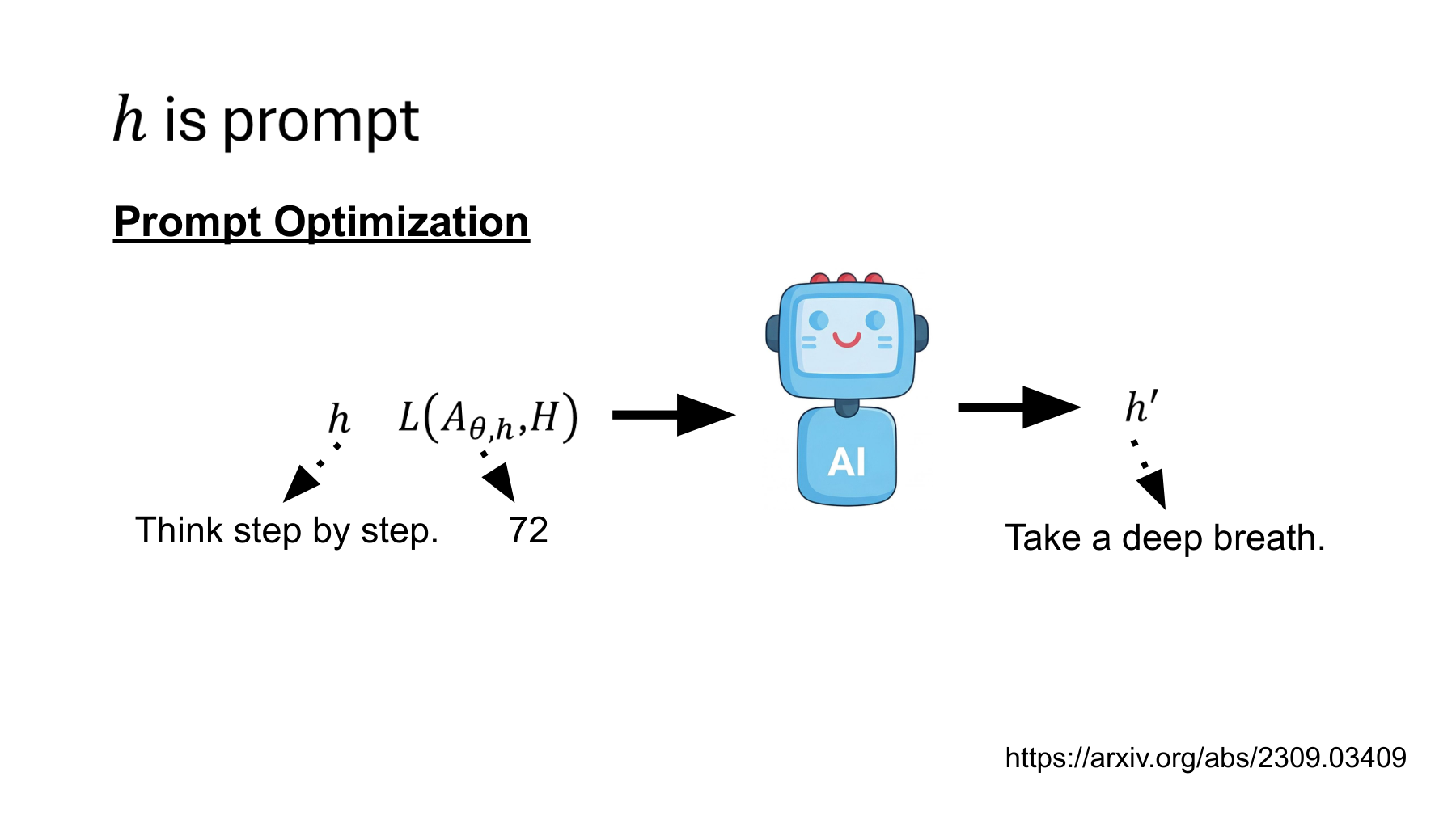
Here the harness is restricted to a prompt. Keep the problem-solving model’s weights fixed and vary the instruction it receives. The lecturer applies an initial instruction to math problems, scores the result, and passes the instruction and score into a separate call requesting a better candidate. Lecture, 8:20–9:44
On the slide, h on the left is the current instruction and h′ on the right is a candidate. The model in the middle proposes candidates. Run the target model again using the new text. The proposer’s confidence cannot determine the evaluation score.
#The model that answers and the model that proposes
The OPRO (Optimization by PROmpting) paper distinguishes two roles. The optimizer LLM proposes instructions. The scorer LLM follows an instruction to answer actual problems. In the math experiments, accuracy comes from comparing those answers with the reference answers. “Scorer” therefore does not mean a model subjectively rating an instruction’s writing style. One base model can fill both roles, but the calls serve different purposes. OPRO, sections 4.1–4.2
Let D be an evaluation set of N questions and record a 0 or 1 for correctness. For a single evaluation with fixed execution settings, the observed accuracy of instruction h is:
| Symbol | Meaning |
|---|---|
| x_i, y_i | The ith problem and its reference answer |
| Aθ,h | A system that runs fixed model θ with instruction h |
| judge | A rule that extracts the answer and checks correctness |
| S(h;D) | Observed accuracy on those questions under the specified conditions |
The intended variable is h. If the judging rule or evaluation items also change, check whether the scores still measure the same thing. For multiple samples per question, specify the number of repeats and aggregation rule. The expression alone does not give expected accuracy over all possible runs.
#Is the 72 in the diagram a loss or a score?
The original figure places L and the number 72 at the evaluation. The lecturer describes 72 as an example benchmark score. Larger OPRO accuracy is better, whereas the losses in earlier parts favor smaller values. Keep the two directions distinct.
For example, assuming 72% accuracy, defining loss as the zero–one error rate gives:
This converts accuracy to error rate. Other losses need not equal one minus a score. Likewise, 72 in the diagram should not be treated as an exact published experimental result.
#What “take a deep breath” means here
The slide’s “Take a deep breath” does not claim that a model breathes like a person to think better. It illustrates a search over input strings and the resulting changes in output distribution and accuracy.
A well-known OPRO comparison used PaLM 2-L on GSM8K with the instruction at the beginning of the answer. Accuracy was 71.8% with the baseline instruction and 80.2% with the discovered one. The difference is 8.4 percentage points, a relative increase of about 11.7%. The result concerns those conditions and does not identify a universally optimal instruction for current models. OPRO, Tables 1 and 4
The transferable idea is the procedure: run candidates on the intended problem, compare them under a shared rule, and apply the selected instruction to new items.
#Second half, slide 12 — Search history enters the meta-prompt
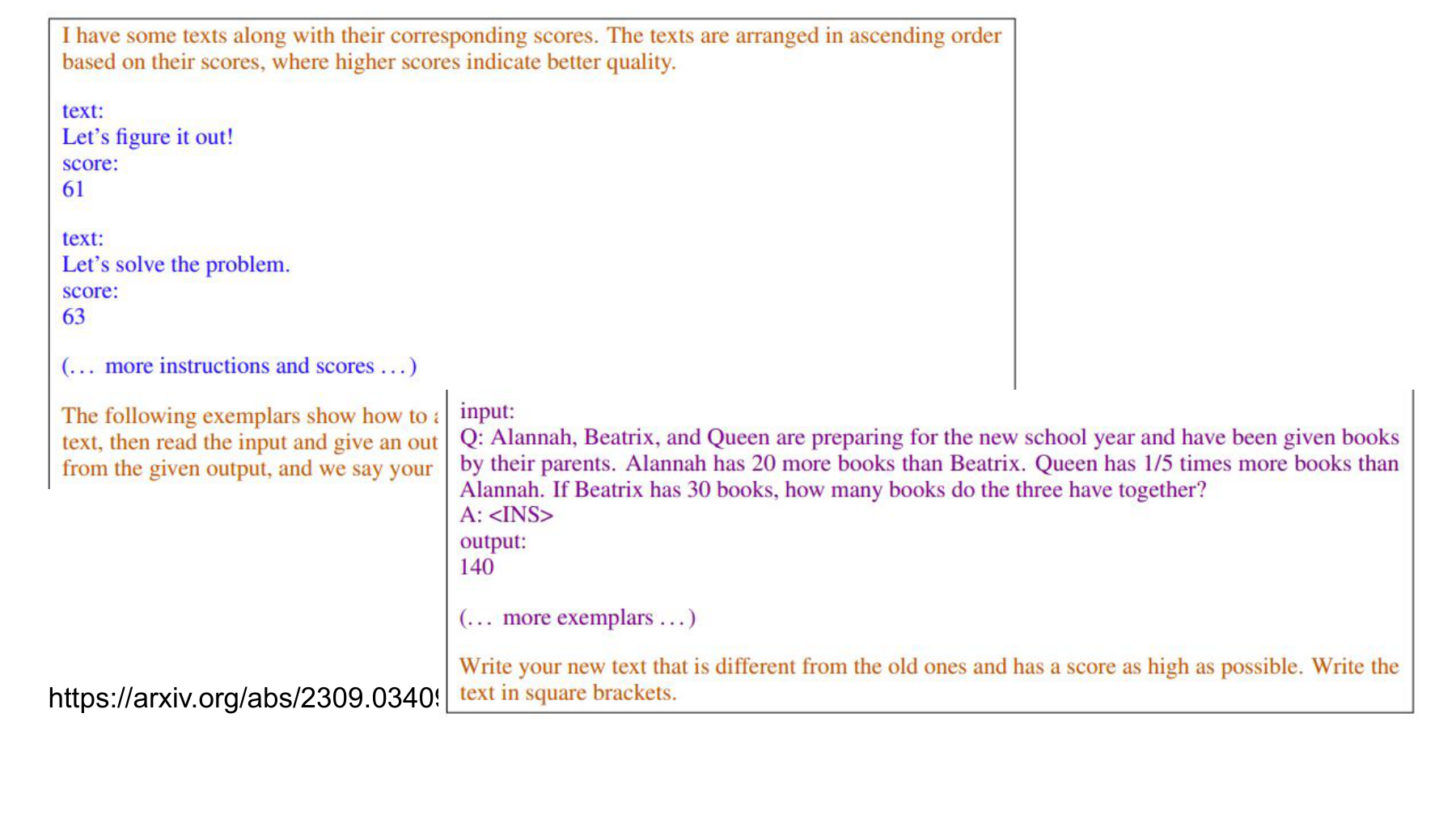
The figure expands the preceding slide’s arrow into an actual input. A meta-prompt asks a model to write instructions for another model. It contains earlier instructions, their scores, example problems, and requirements for producing a new candidate. Lecture, 9:44–10:27
Each element has a distinct function. Example problems show the task. The insertion point shows the context in which the new instruction will appear. Candidate and score history records directions already explored. An output format lets the next evaluation consume the candidate. Assembling this input is itself harness design.
This reduces the need for a person to write a finished instruction from scratch. Someone must still define the problems, scoring function, number of candidates, and search budget. Inspect candidates for repeated wording or answers to individual examples embedded in the instruction.
#A related CMU lecture — Feeding evaluation results into the next proposal
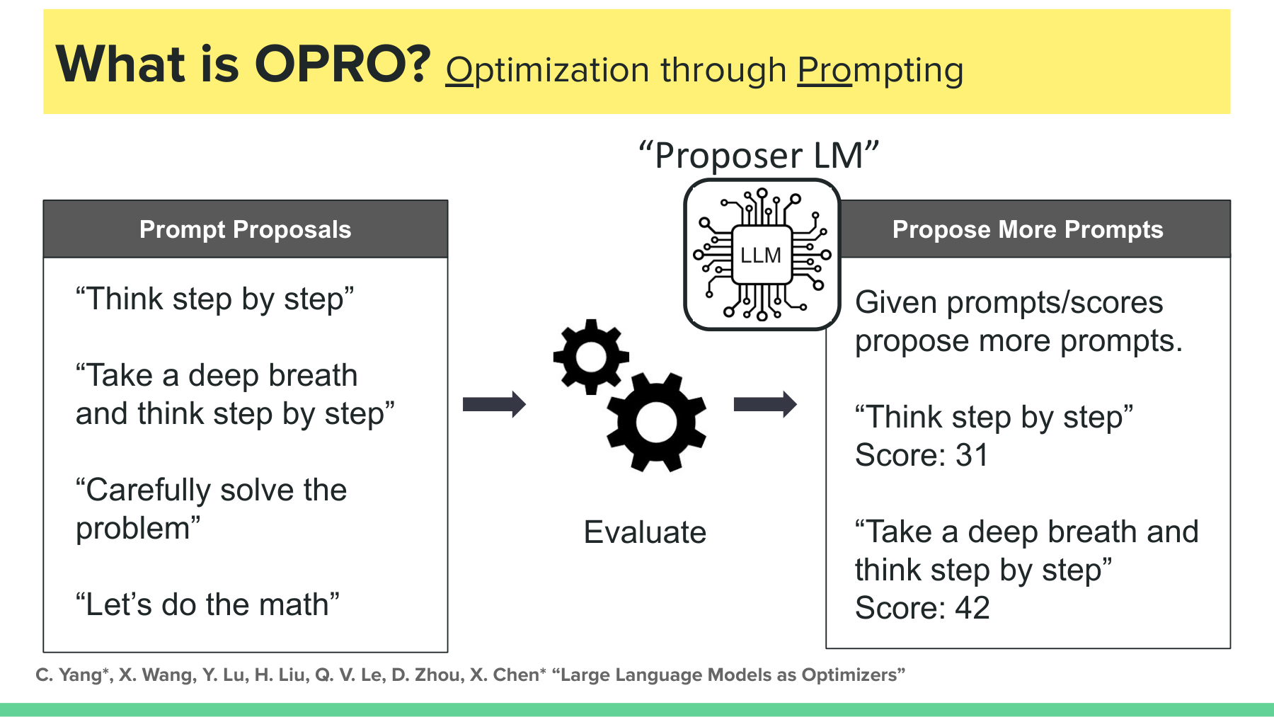
Reading left to right, candidates pass through the evaluator first. The candidate text and measured values then enter the proposer LM. The 31 and 42 in the diagram illustrate this connection and are separate from the GSM8K table discussed earlier. CMU, slide 58
Suppose a data extraction agent is optimized against an evaluator that checks only JSON format. Search may favor a candidate that emits valid JSON more often. Whether the dates and names inside are accurate is a separate condition. Repeated feedback steers search toward the objective expressed by the evaluator. In this example, both format pass rate and content accuracy need definitions.
The next lecture segment contrasts replacing a single candidate in sequence with keeping several candidates. OPRO itself retains previous high-scoring instructions and generates multiple candidates per step. Describing all of OPRO as keeping only its last instruction would be incorrect. GEPA’s distinctive features include how it uses execution feedback and how it selects future parents. OPRO, sections 4.2 and 5.1
#Worked example 1 — Search scores and selection scores
The following hypothetical experiment illustrates data roles. It uses 50 fit items for candidate generation and 50 validation items for selection. The split differs from the original OPRO experiment.
| Candidate | Correct on fit | Fit accuracy | Correct on validation | Validation accuracy |
|---|---|---|---|---|
| A | 34/50 | 68% | 35/50 | 70% |
| B | 39/50 | 78% | 40/50 | 80% |
| C | 41/50 | 82% | 33/50 | 66% |
C has the highest fit score. If the predetermined rule maximizes validation accuracy, choose B.
C’s scores differ across the two sets. A single result on 50 items cannot establish that overfitting caused the gap. Item composition and run variability may also contribute. Now freeze B and suppose baseline A answers 34 of 50 previously unused test questions correctly, versus 38 for B.
The eight-point difference is an observation on this test set. It does not alone establish statistical significance or deployment gains elsewhere. If the test result informs further edits to B, that test set has participated in search.
OPRO also discusses prompt-search overfitting. Its default setting uses no separate validation set, and a further analysis investigates using one. The splits above illustrate a comparison design for this article. OPRO, section 5.4
#Which items changed behind an eight-point gain?
The evaluator on CMU slide 58 returns one score per candidate. That score can guide the next proposal. To investigate whether the new instruction broke previously correct answers, retain the item-level predictions as well. In the hypothetical 50-item test above, suppose both instructions get 30 right, only A gets four right, only B gets eight right, and both miss eight. CMU, slide 58
Items that both candidates solve or both miss cancel in the difference. B repairs eight failures and introduces four errors. If all four new errors involve unit conversion, those items suggest a specific diagnostic case for the next meta-prompt. The decomposition requires matching item IDs, answer keys and model settings. Once these 50 items inform another edit, use a fresh holdout to report final performance.
#Where does search incur costs?
In a separate hypothetical example, evaluate eight candidates on 25 problems each and two finalists on 100 each. With one target-model call per problem, the number of target-model runs is:
This excludes calls for proposing candidates or diagnosing failures, retries, and tool execution. Even 400 calls can have different token costs depending on input and output length. To understand the resources needed for a fixed-weight method, separate the cost of finding a prompt from the cost of running it in a service.
#Second half, slide 13 — GEPA uses failure traces and complementary strengths
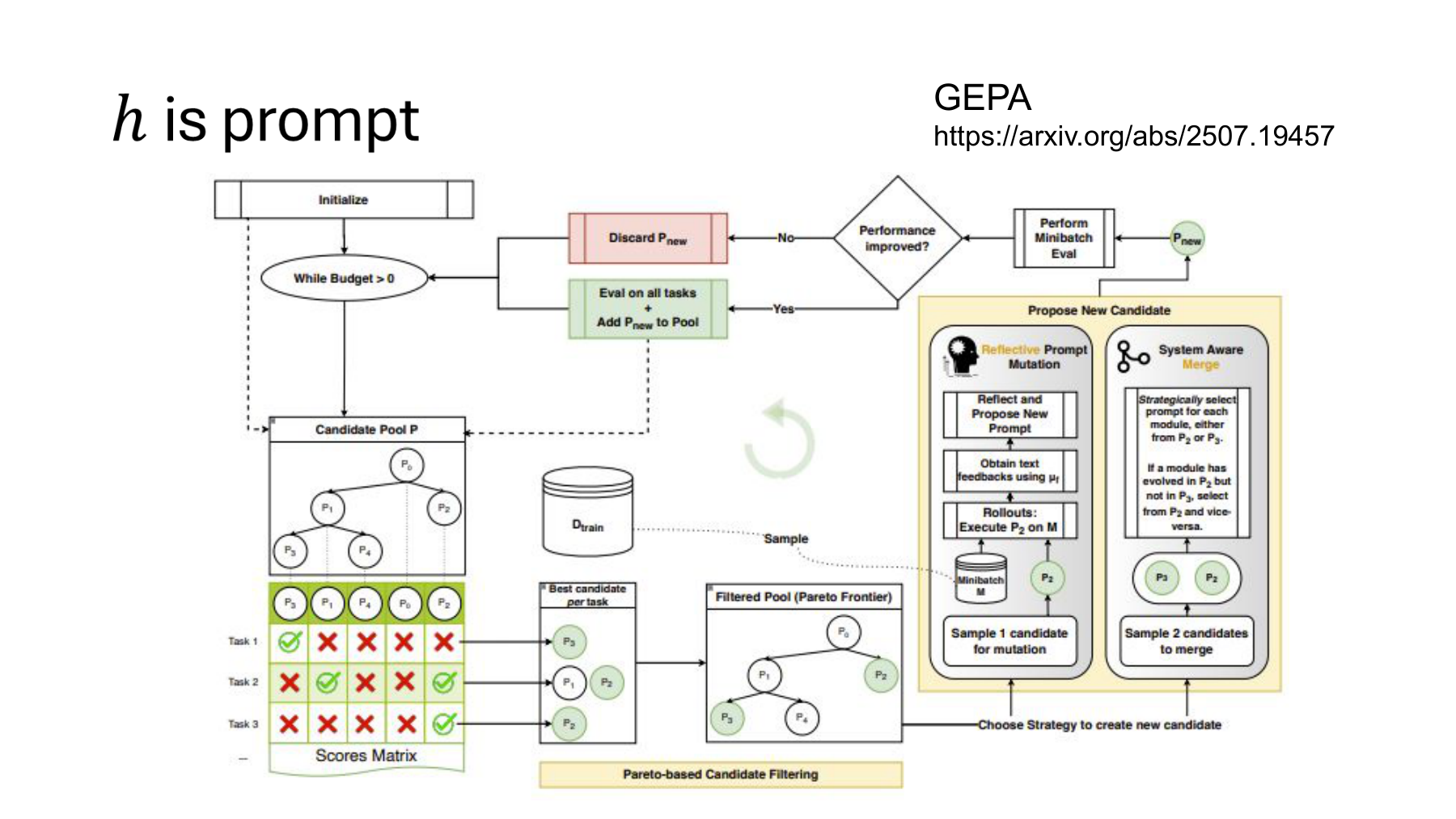
Read the diagram in three parts. The left shows how the starting candidate is chosen, the right how it is revised, and the top how revisions are evaluated. The NTU lecture also distinguishes mutating a single candidate from combining two. Lecture, 12:59–13:53
GEPA (Genetic-Pareto) runs a prompted program and searches its inputs, outputs, tool responses, and errors for clues to a revision. The program may contain several LLM modules. After editing a selected module’s instruction, rerun it with the other modules to measure overall performance. The original prompt optimization procedure fixes base-model weights. GEPA, sections 2–3
#A related Stanford talk — Identical zeros can carry different information
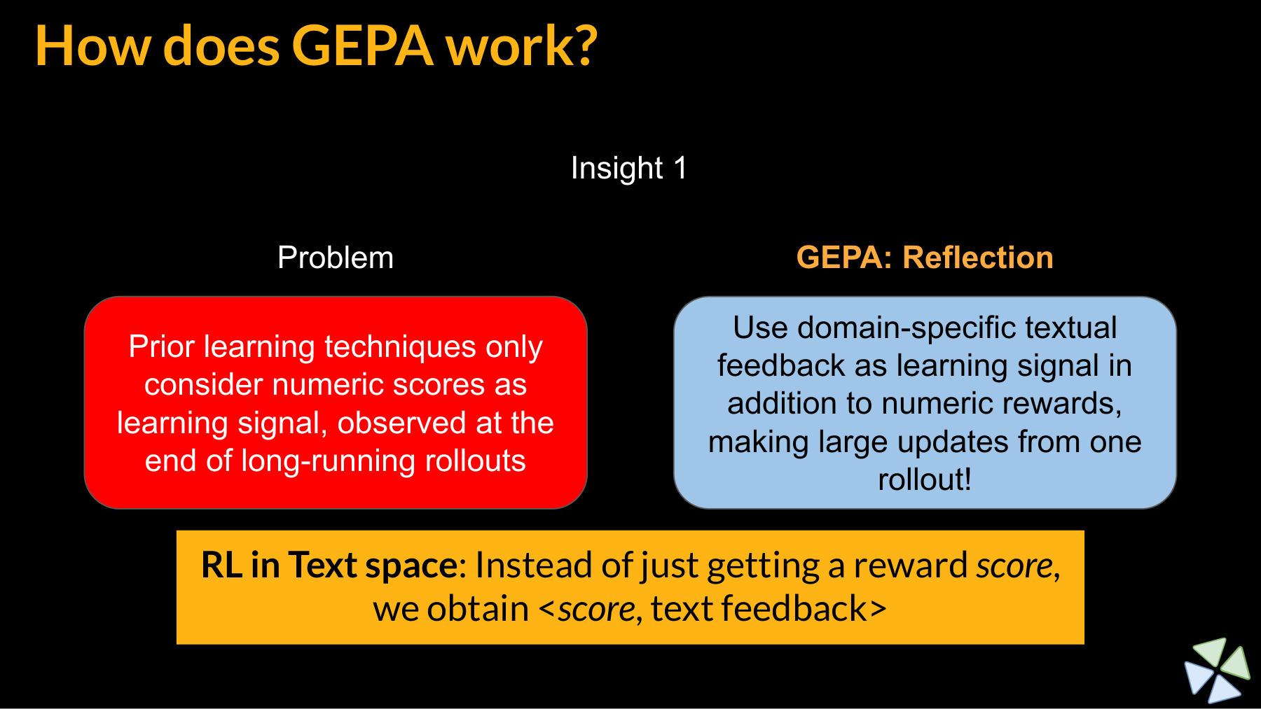
The slide emphasizes how much information feedback carries. A zero tells us a run failed. Knowing which tool call failed or which input format was invalid gives the next proposal a direction. In a subsequent ICLR presentation, the author gives the example of a compiler reporting an unavailable API. A reflection model can use the trace to propose an alternative API. ICLR talk, 2:25–2:58
Suppose three code runs fail with the following records. The entries are illustrative.
| Final score | Trace detail | What to examine in the next candidate |
|---|---|---|
| 0 | Function name not found | Available APIs and versions |
| 0 | Correct result, but the output parser failed | Output format and unnecessary explanatory text |
| 0 | Editing started before the necessary file was read | Order of inspection and editing |
These traces can produce more specific candidates than “answer more accurately.” The model’s diagnosis remains an inference. Run the revision to check whether it reduces the failure and whether it breaks previously successful cases.
The slide describes this intuitively as reinforcement learning in text space. Here that means reading feedback and searching over natural-language instructions. It makes no general claim that all RL uses a single number, or that GEPA performs the gradient update used by GRPO.
#How candidates are generated and checked
GEPA’s main steps are described in Algorithms 1–2 and the authors’ talk, 5:24–6:17.
- Select a parent candidate and a module to revise.
- Collect traces and scores on a small batch of feedback examples.
- Have a reflection model read this information and propose a new instruction.
- Compare parent and candidate on the same small batch.
- Evaluate an improved candidate on the selection items and record its scores in the matrix.
The combination route also considers which changes to inherit from each module. Concatenating two strings does not guarantee the corresponding functions will work together. Because the selection items repeatedly influence parent choice, reserve separate data for reporting final generalization.
#A related Stanford talk — A lower average can still be valuable for search
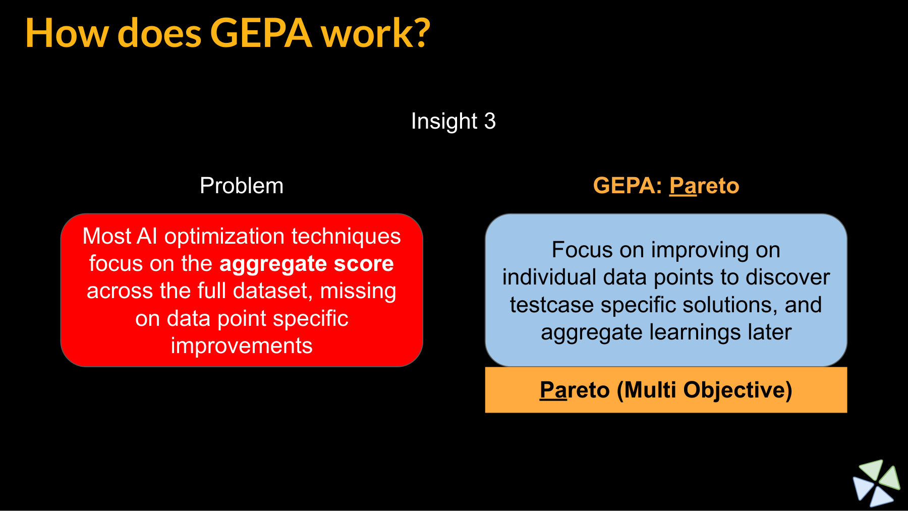
A candidate’s mean score obscures which problems it solved. If it solves a problem the average leader struggles with, it can still contribute to a later revision. In a follow-up talk, the author explains how preserving per-item strengths allows rare solutions to reach later candidates. ICLR talk, 6:54–7:24
GEPA implements the idea with a per-item score matrix and a parent-selection procedure. To understand the search, start by treating each item as a separate performance dimension. A two-axis cost–accuracy Pareto plot illustrates a different comparison.
#Worked example 2 — Calculating selection by item
This hypothetical score matrix covers three equally weighted items and four candidates. Scores span 0–1 and can take intermediate values as well as binary correctness values.
| Candidate | Item 1 | Item 2 | Item 3 | Mean score |
|---|---|---|---|---|
| A | 0.90 | 0.80 | 0.20 | 0.6333 |
| B | 0.40 | 0.30 | 0.95 | 0.5500 |
| C | 0.60 | 0.60 | 0.60 | 0.6000 |
| D | 0.70 | 0.50 | 0.10 | 0.4333 |
A leads on mean score, but B leads on item 3. Write s_k[i] for candidate k’s score on item i. The set of leaders on each item is:
Only A leads on items 1 and 2, and only B leads on item 3. Their union is A and B. Algorithm 2 removes dominated candidates within this union, then samples a parent in proportion to how often each candidate appears among the per-item leaders. Neither A nor B dominates the other here.
B can therefore become a parent despite having a lower mean than A. These probabilities describe parent selection in this example. The one-third probability for B does not describe its chance of producing a better descendant.
Under the usual definition of Pareto dominance, a candidate is dominated if another is at least as good on every item and strictly better on at least one. C is also nondominated: A scores lower on item 3 and B scores lower on items 1 and 2. C leads on no item, so it falls outside the union of per-item leaders.
Thus the general nondominated set is A, B, and C, while the GEPA parent-selection set in this example is A and B. A dominates D on every item. The algorithm differs from uniformly sampling all nondominated candidates. Exclusion from this parent-selection step does not imply permanent deletion from the candidate record. GEPA, Algorithm 2
#What can the screening batch miss?
Figure 3 of GEPA shows two evaluations. A mutation that improves on its parent on a small batch gets evaluated on a larger validation set and enters the pool. How can that cheap screen miss regressions? In this invented example, a proposed instruction gains 0.2 on each of three items, loses 0.4 on each of two, and leaves five unchanged. GEPA, Figure 3, page 5
Sample three of the ten uniformly without replacement. There are 56 triples among the eight non-regressing items. Ten of those triples contain only unchanged items. The other 46 reveal at least one improvement and no losses.
Although the full mean declines, this batch shows a strict improvement and advances the candidate about 38.3% of the time. Two gains and one loss sum to exactly zero and fail the strict screen. The probability follows from this particular item mix and sampling rule. The paper’s search procedure supplies the comparison rule.
#What do GEPA’s results establish?
In the paper’s Qwen3-8B comparison, GEPA averages 54.85 over six tasks and GRPO averages 48.91. On AIME-2025 in the same table, GRPO scores 38.00 against GEPA’s 32.00. “Can Outperform Reinforcement Learning” in the title refers to experimental settings where GEPA performs better, not a universal ranking. GEPA, Table 1 and section 4
Fewer rollouts do not necessarily lower total cost by the same factor. Include reflection-model calls, trace lengths, and candidate evaluation coverage. For a comparison on your own system, match the base model, items, judging rules, and the scope of costs counted.
#Second half, slide 14 — ALMA changes the design that manages memory
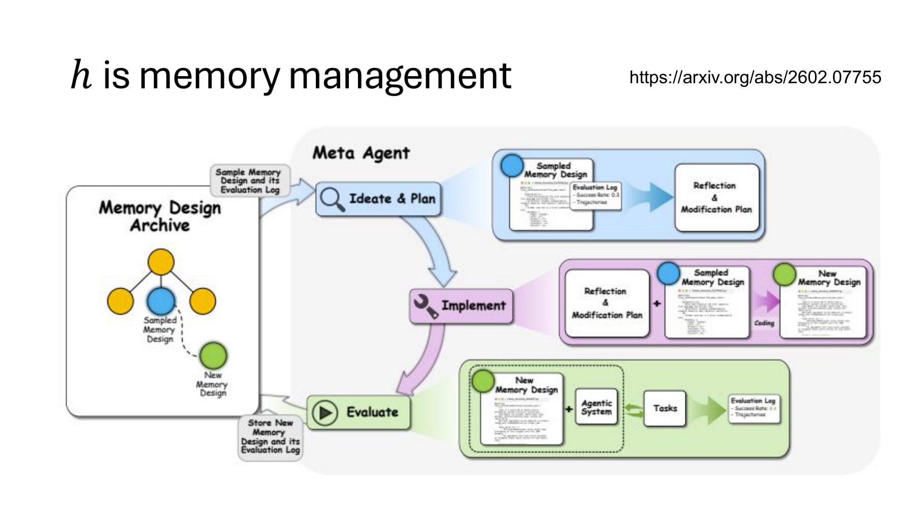
The target now moves from instructions to memory management. To use experience, an agent needs rules for deciding what to store, how to organize it, and what to retrieve for the current task. The NTU lecture introduces a method that generates and evaluates candidates for this design. Lecture, 13:53–15:31
ALMA stands for Automated meta-Learning of Memory designs for Agentic systems. Its meta-agent reads existing memory design code and evaluation logs and implements a new design. Evaluation connects the design to a fixed task agent. The paper’s main interfaces are general_update() and general_retrieve(). Their code defines the storage structure and procedures for updating and searching it. ALMA, sections 3.1–3.3
#Memory contents and memory design are distinct
Memory contents are the experiences accumulated so far. Memory design is the code that determines how to store and retrieve those experiences.
Write M for the contents and φ for the design. Here φ identifies memory code, with no assumption that it is a continuous vector of neural weights. With τ_t denoting the agent’s trace and q_t the current problem, update and retrieval can be written as:
U_φ determines which experiences to store and how. R_φ retrieves material z_t for the current problem. Adding a record under fixed φ changes the contents under the same design. Editing the retrieval rule or storage code to form φ′ changes the design itself. Both can change simultaneously, so specify which level is under evaluation.
| Change | Quantity changed | Example |
|---|---|---|
| Experience accumulation | M | Store a failed API call and the conditions that resolved it |
| Retrieval result | z_t | Retrieve an earlier error relevant to a new question |
| Memory design improvement | φ | Change code to store version and environment conditions and use them in retrieval |
These API examples are illustrative. A previously successful command can fail under a new version. Storing applicability conditions alongside successful commands may help, but longer records are not invariably better. Evaluate missed records and failures to account for obsolete conditions.
#Using experience in the inner loop and searching designs in the outer loop
In the figure’s inner loop, the agent uses memory while doing tasks. In the outer loop, the meta-agent reads scores and logs and revises memory code. To read ALMA, track both what was remembered and the design that determined how it was remembered.
The experimental design separates these levels. ALMA first gathers experience to build memory, then tests its usefulness on later tasks. During design search, static mode fixes memory during the deployment period. Testing the selected design also includes dynamic mode, which continues updating the contents. Even in static mode, the update function builds memory during the earlier collection phase. ALMA, section 3.2
In a general experiment, preloading two designs with different experiences confounds design with experience. If B remembers the answers to test questions it solved earlier while A starts empty, the comparison is unfair. Specify the data used to collect experience, initial state, problem order, and whether memory updates during deployment. These are comparison principles derived from the architecture.
#Reading the paper’s results — Average improvement and individual conditions
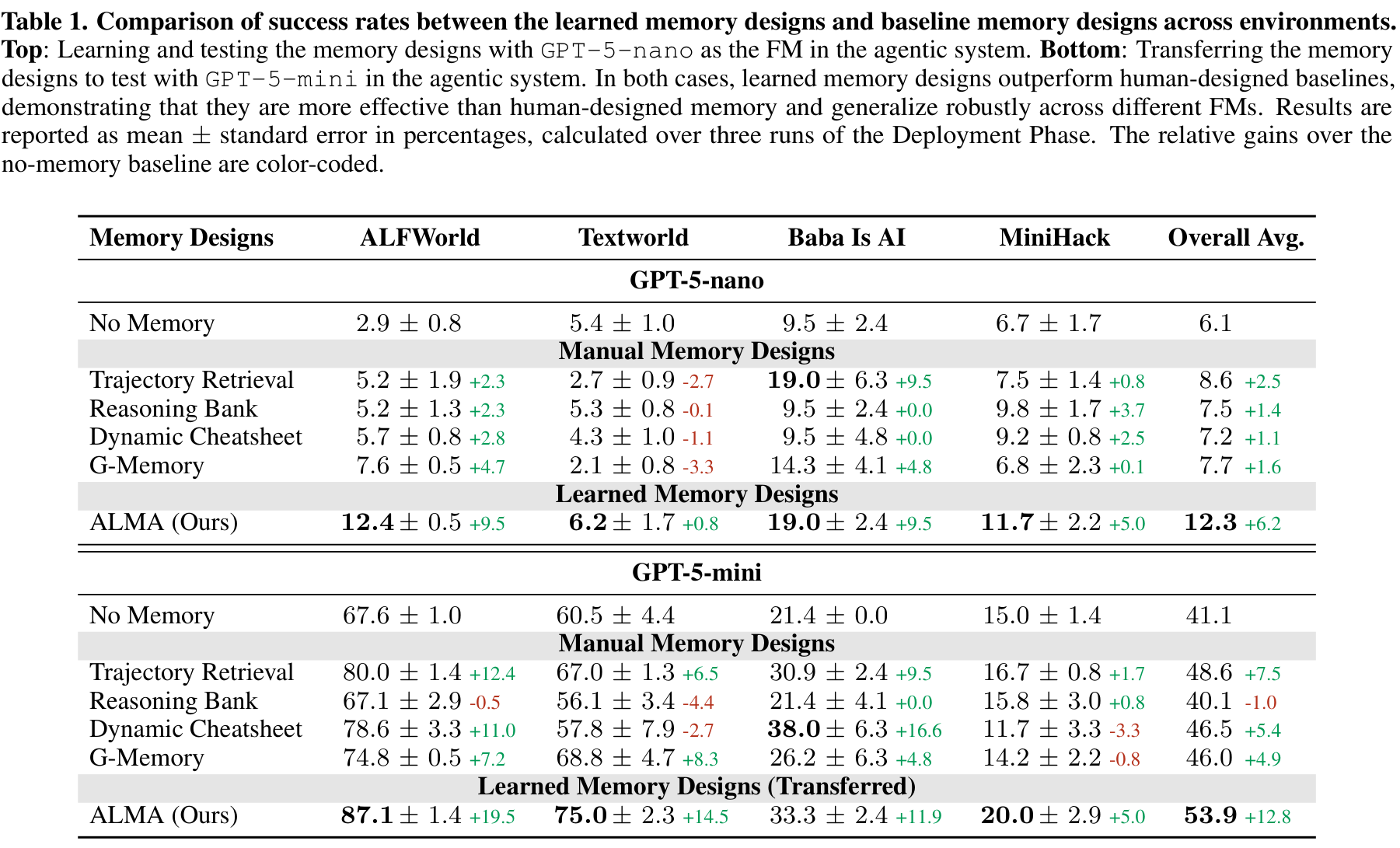
The table covers ALFWorld, TextWorld, Baba Is AI, and MiniHack. In the displayed overall averages, GPT-5-nano rises from 6.1% without memory to 12.3% with ALMA, and GPT-5-mini from 41.1% to 53.9%. Subtracting the displayed values gives 6.2 and 12.8 percentage points, respectively. Per-environment error bars are standard errors across three deployment runs. ALMA, section 4.1 and Table 1
On Baba Is AI with GPT-5-mini, Dynamic Cheatsheet scores 38.0% versus ALMA’s 33.3%. The mean gain does not establish a win over every baseline in every environment. Individual cells are already rounded, so averaging them may differ in the final digit from averaging the underlying data.
The research question is more specific than whether memory capacity can grow: Can we find storage, update, and retrieval rules that let the same agent use experience more effectively? In your own system, examine success rate alongside retrieved context length, storage and retrieval cost, and failures due to stale experience.
#When does a different memory design win?
ALMA Figure 4 varies the number of trajectories available during collection, then freezes the memory during evaluation. This isolates the value of the collected memory from any further writes during deployment. Figure 5 asks a separate question about a shift in the deployment task distribution. Consider the following invented inspection-equipment example. ALMA §3.2 and Figures 4–5
Test memory designs U and V on the same held-out tasks. There are ten routine setup problems and ten unfamiliar diagnostic problems. U solves eight setup and four diagnostic problems, while V solves six setup and seven diagnostic problems. Let q be the fraction of setup requests in deployment. The expected success rate weights the two within-type rates by the incoming mix.
With an even mix, U scores 60% and V scores 65%. With 80% setup requests, U scores 72% and V scores 62%. The ranking changes because the task mix changes. This calculation assumes the within-type rates hold after deployment. A shift in difficulty within either type calls for a new measurement there.
#Second half, slide 15 — DGM edits the agent’s own code
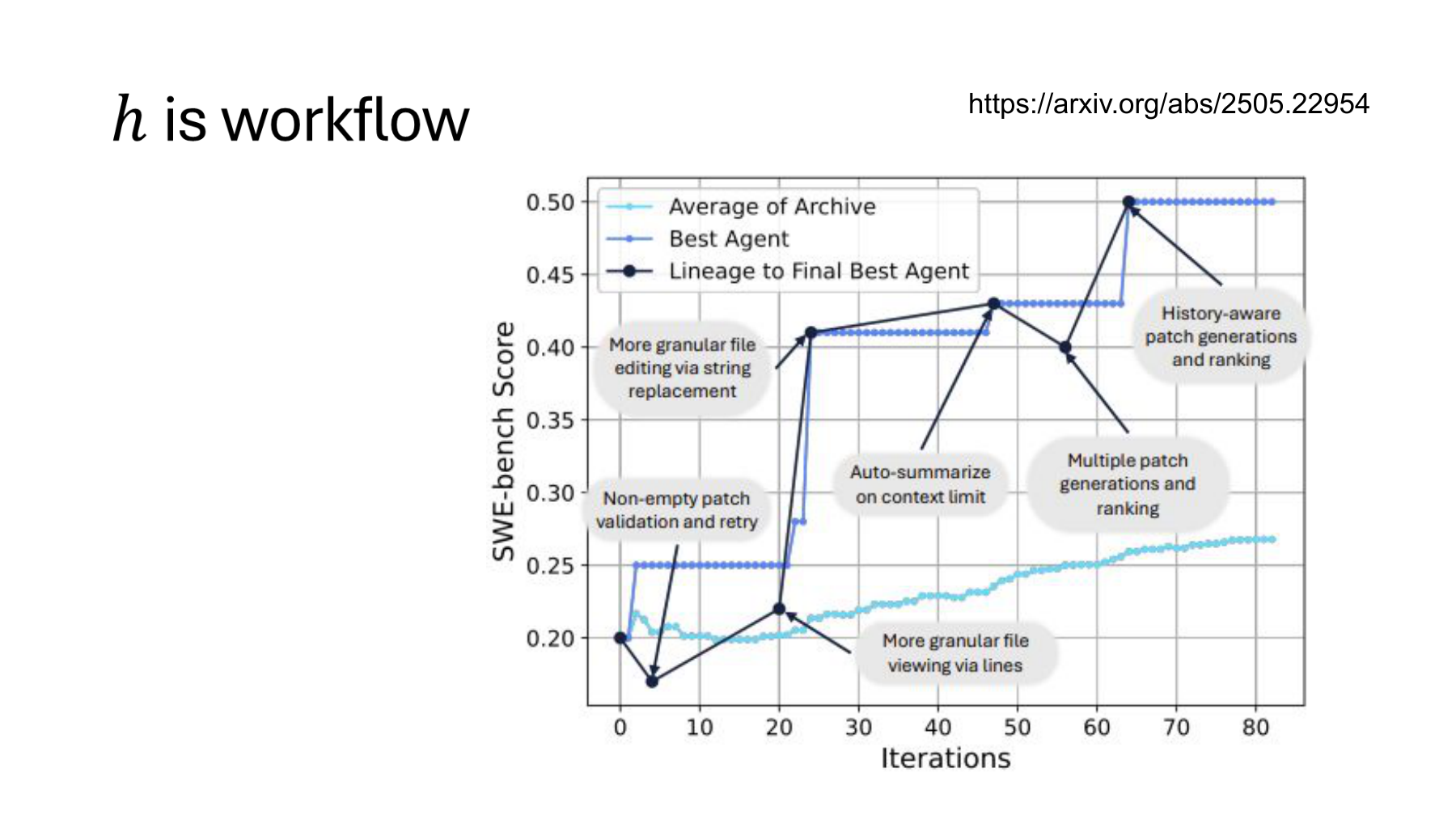
Here the harness h extends to workflow. Graph annotations include tools for reading specified lines of a file and editing by string replacement, and a procedure for summarizing long contexts. The lecturer presents these as changes to the agent’s own way of working. Lecture, 15:31–17:12
The Darwin Gödel Machine (DGM) modifies the coding agent’s own code. An agent’s ability to edit a repository for an external task also lets it edit its own tools, instructions, and execution procedures. The base-model weights stay fixed, and candidates with modified code are evaluated on coding benchmarks. DGM, section 3
Editing a function in an external project changes that project. Adding a file-editing tool to the agent’s own code changes the harness used on later tasks. Both operations write code. Following where the change persists distinguishes solving a task from improving the system.
#Reading the three curves separately
The figure shows three different aggregates. DGM, Figure 3 and caption
| Curve | Meaning |
|---|---|
| Light blue | Mean score of retained candidates |
| Blue | Score of the best candidate discovered so far |
| Dark line and points | Ancestral path to the final best candidate |
A rise in the best score does not make every revision successful. If a new candidate underperforms but the archive retains the previous best, the record still stands. A dip in the ancestral path shows how a weaker candidate can become the starting point for later search.
Consider a hypothetical archive with fixed evaluation rules and fixed recorded scores. Let ℋ_t be the candidate set at time t. Its best score and mean are:
When earlier candidates are retained and a new one is added, the record cannot decline.
That follows from the maximum of a set, regardless of whether a new candidate is better. Add a candidate scoring 0.2 to scores of 0.4 and 0.3: the best stays at 0.4 while the mean falls.
The record, distribution of candidate scores, and lineage used for further search therefore answer different questions. The equations assume fixed scores. When actual experiments remeasure performance using a different dataset or repetition count, account for measurement variation.
#Performance and the scope of self-modification
DGM reports an increase from 20.0% to 50.0% in its SWE-bench experiment. This comparison uses a 200-item subset of SWE-bench Verified, out of the full 500 items. Candidates were not all evaluated on equal numbers of tasks during search. The procedure starts with small sets and evaluates promising candidates on larger ones. DGM, sections 4.2–4.4
The gain is 30 percentage points, and the final score is 2.5 times the initial score. This describes the coding system under those evaluation conditions and gives no equivalent multiplier for the intelligence of the model weights. On Polyglot, the paper distinguishes 14.0%→38.0% on the search subset from 14.2%→30.7% on the full benchmark. Same section
Despite “Gödel” in the name, DGM does not mathematically prove that every edit is beneficial. It tests changes empirically. Its self-modification scope is explicit: the outer search process, including archive maintenance and parent selection, stays fixed. The agent cannot freely rewrite every evaluation and search rule in this implementation. DGM, section 3
DGM also retains more than just candidates that outperform their parents. Candidates that preserve basic code-editing capabilities can enter the archive, and a low-scoring candidate may lead to a useful change later. The next part examines this retention policy and actual lineages in more detail.
#Reading the four methods through a common question
Across these five slides, the scope of the harness has expanded. The table makes “the system improved itself” more precise by identifying what the system actually did.
| Method | Target | Evidence for revision | Evaluation distinction |
|---|---|---|---|
| OPRO | Instructions | Previous candidates and task scores | Generation data vs. final test data |
| GEPA | Module prompts | Execution traces, textual feedback, and per-item scores | Parent selection vs. final evaluation |
| ALMA | Memory storage, update, and retrieval code | Performance using experience and execution logs | Changes to contents vs. changes to design |
| DGM | The agent’s own code and workflow | Coding task evaluations and candidate history | Modifiable code vs. fixed outer search |
To adapt these methods, first make the file or instruction under revision identifiable as a specific version. Set the evaluation tasks, execution conditions, and costs to count. Give the proposer the information needed to revise, and test the selected revision on new problems. This ties the result to a specific system and change.
A longer prompt or larger memory does not establish better performance. Compare accuracy, cost, and failure types together. As the examples show, per-item results reveal things the mean can hide, and intermediate candidates carry information distinct from the best-so-far record.
Part 17 starts with slide 16. It follows the candidates DGM retained and the paths that produced their descendants before turning to links between program-level optimization and model training.
Calculations and code
The code calculates accuracy and error rate, candidate selection, execution budgets, per-item leaders and general nondominated sets, parent-selection probabilities, and archive maxima and means. Small examples check ties and removal of dominated candidates. It distinguishes arithmetic checks on published results from hypothetical examples and does not run models or reproduce benchmarks. It also records differences between ALMA’s displayed averages and averages recomputed from rounded cells.
#Further reading
| Resource | Relevant topic |
|---|---|
| NTU second lecture, slides 11–15 · Lecture video | Harness improvement from prompts to memory and workflows |
| OPRO, arXiv v3 | Meta-prompts based on candidate histories and scores, and analysis of overfitting |
| CMU LLMs lecture, slide 58 | The roles of the proposer and evaluation loop |
| GEPA, arXiv v2 | Execution feedback, module-level revisions, and the per-item parent-selection algorithm |
| Stanford GEPA talk, slide 27 · Slide 31 | Textual feedback and preserving strengths on individual items |
| GEPA authors’ ICLR 2026 talk · 2:25 · 5:24 · 6:54 | API errors, data splits, and per-item candidate selection and combination |
| ALMA, arXiv v1 | Using memory contents and searching memory design code |
| Darwin Gödel Machine, arXiv v3 | Editing agent code, archiving candidates, evaluation scope, and boundaries of self-modification |
For OPRO, this article uses the 2024 v3 of work first released in 2023. The cited versions of GEPA, ALMA, and DGM appeared in February, February, and March 2026, respectively. The Stanford slides are from a 2025 talk. The ICLR video is a separate later presentation. Performance numbers are from the specified versions.