AI self-evaluation, agreement across answers, and high confidence can all supply learning signals. Improving a signal alone does not establish that answers became more accurate.
Part 5 — AI That Designs Rewards and AI That Evaluates Answers distinguished reward-code design from answer-quality evaluation. We now ask what signals a model can construct from its outputs without ground-truth answers for evaluation. The phrase “AI grades itself” covers three different methods.
One is verbal self-evaluation with scores. Another is aggregation across repeated answers to find agreement. The third is entropy, which measures how concentrated an output distribution is. They use different information and calculations. Also check whether a method changes only the chosen answer or updates network parameters as well.
Questions by slide
| Slide | Question |
|---|---|
| 26 | What roles do the answer generator and the evaluator supplying a loss perform? |
| 27 | How does a score of 5 differ from the probability of the “Yes” token? |
| 28 | When does a majority answer become a pseudo-label, and when is it actually used in training? |
| 29 | What does lower entropy mean, and what does it leave uncertain? |
| 30 | What does entropy minimization change in images, speech, and language? |
#Slide 26 — Producing an answer and producing an evaluation signal
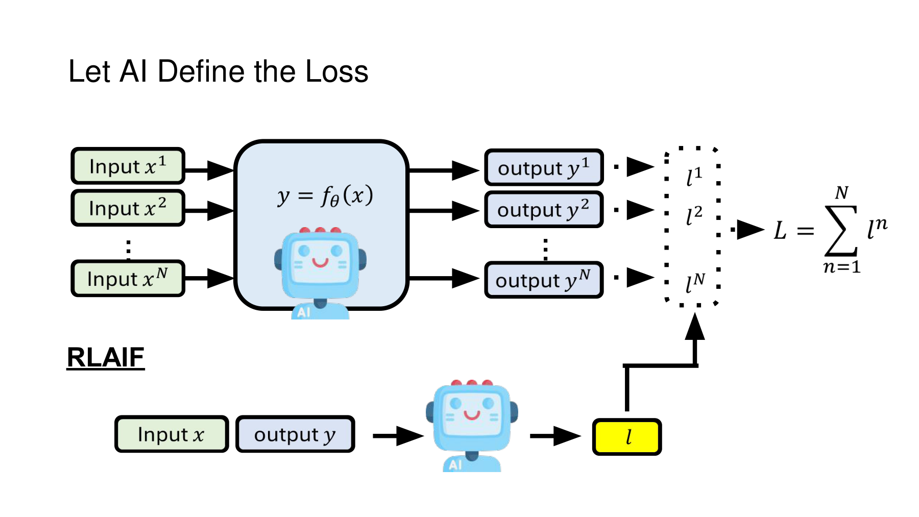
At the top, the slide shows inputs, model outputs, individual losses, and their sum. The lower RLAIF diagram passes the input and answer to an evaluator and turns its judgment into a loss. These five slides develop the question of what can supply an evaluation signal when ground-truth labels are not always available.
#Matching AI icons need not mean matching parameters
Denote the question by , the answer by , and the generation policy by . The policy generates an answer, while the evaluator receives the question and answer and computes a score or loss. The following notation distinguishes their roles.
denotes evaluator parameters and its criteria or instructions. The last function maps a score to a loss for the training objective. For example, if a higher score is better, minimizing a loss requires changing the sign or reference point.
The generator and evaluator can use the same type of model, different models, or identical weights under different prompts. Identical robot icons on the slide do not establish shared parameters. Conversely, different model names do not establish independent errors. In a real system, inspect models, prompts, training data, and evidence available to the evaluator.
The distinction from Part 5 still applies. Scoring an answer highly, using the assessment to create training data, and updating a generative policy are separate stages. Calculating a score alone does not train the generator.
#A missing answer label does not imply missing criteria
AI evaluation can supply a useful signal for tasks with explicit criteria, such as obeying a format or including required items. For calculation or knowledge problems the model finds difficult, repeated self-evaluation can repeat the original error. Reliability depends on both the task and the evidence supporting the judgment.
Alongside “Did it use external labels?” ask what prior knowledge and evaluation criteria were already present, what was learned from new inputs, and how improvement was tested. A pretrained model and human-written criteria already supply information to the process.
#Slide 27 — Distinguish verbal scores from token probabilities
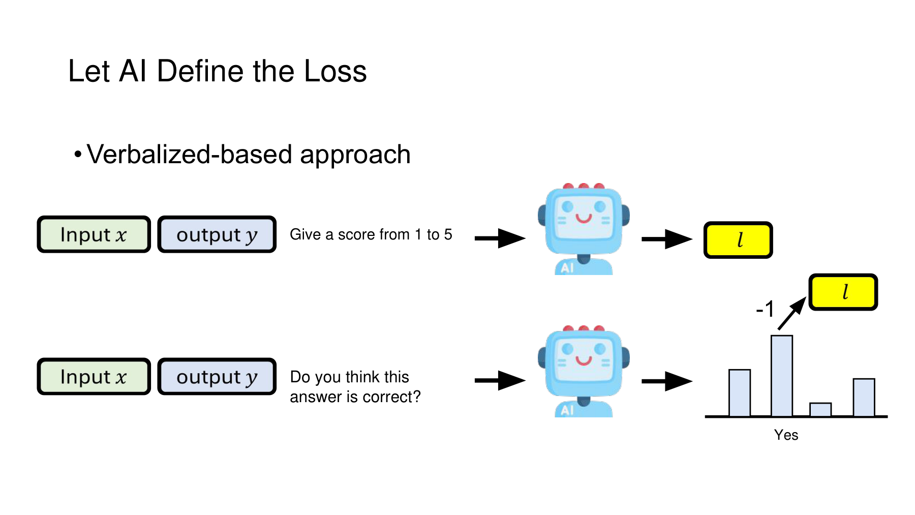
The slide presents a verbalized evaluation approach. Above, the evaluator rates an answer to a given input on a 1–5 scale. Below, it is asked whether the answer is correct, and the probability of a “Yes” response enters the loss. The −1 draws attention to the sign that converts high affirmative probability into low loss.
#A 1–5 rating is a number, but it need not be a probability
Suppose the evaluator gives score according to its criteria. If a higher score indicates a better answer, one possible loss is the following. This illustrates the principle and is not a universal RLAIF loss.
If answers A and B score 4.5 and 2 in a hypothetical example, their losses are 0.5 and 3. Minimizing prefers A. Calling the score itself a loss and minimizing it would push good answers toward lower scores. Evaluation scores, rewards, and losses cannot simply be renamed and optimized in the same direction.
A rating of 4 also does not mean an 80% chance of correctness. A 1–5 scale depends on how it combines factuality, fidelity, brevity, and other criteria. Treating a move from 1 to 2 as equal in size to one from 4 to 5 is a further design choice. Numeric output alone determines neither scale meaning nor calibration.
#An affirmative statement and the probability of generating it
The lower figure uses the affirmative response probability under an evaluation prompt. Take the simple case in which “Yes” is one token.
This notation explains the minus sign. A higher probability of “Yes” gives lower loss. But this is the probability of generating a particular response under a given prompt. Interpreting it as a probability of correctness needs separate validation.
Actual affirmative responses may use “Yes”, “ yes”, or “Correct”. A tokenizer may split a word into several tokens. Renormalizing only Yes and No gives a value different from the Yes probability over the full vocabulary. If the model outputs the string “90% confident,” distinguish the number in the string from the probability of generating the string.
A math evaluator might assign a high affirmative probability to a polished explanation. Recomputing the answer supplies different evidence. Check how the evaluation signal relates to accuracy on separate data with ground truth.
#Using evaluation for selection or for training
Generating several candidates and returning the highest scoring one is reranking. This alone leaves weights fixed. A training stage can store high-scoring answers as targets for subsequent learning or update the policy using scores as rewards.
Verify “the evaluator selected a better answer” separately from “the generator changed so it produces better answers to future questions.” Additional compute for selection should also be accounted for when attributing gains to the model.
#Slide 28 — Agreement is useful evidence but does not certify correctness
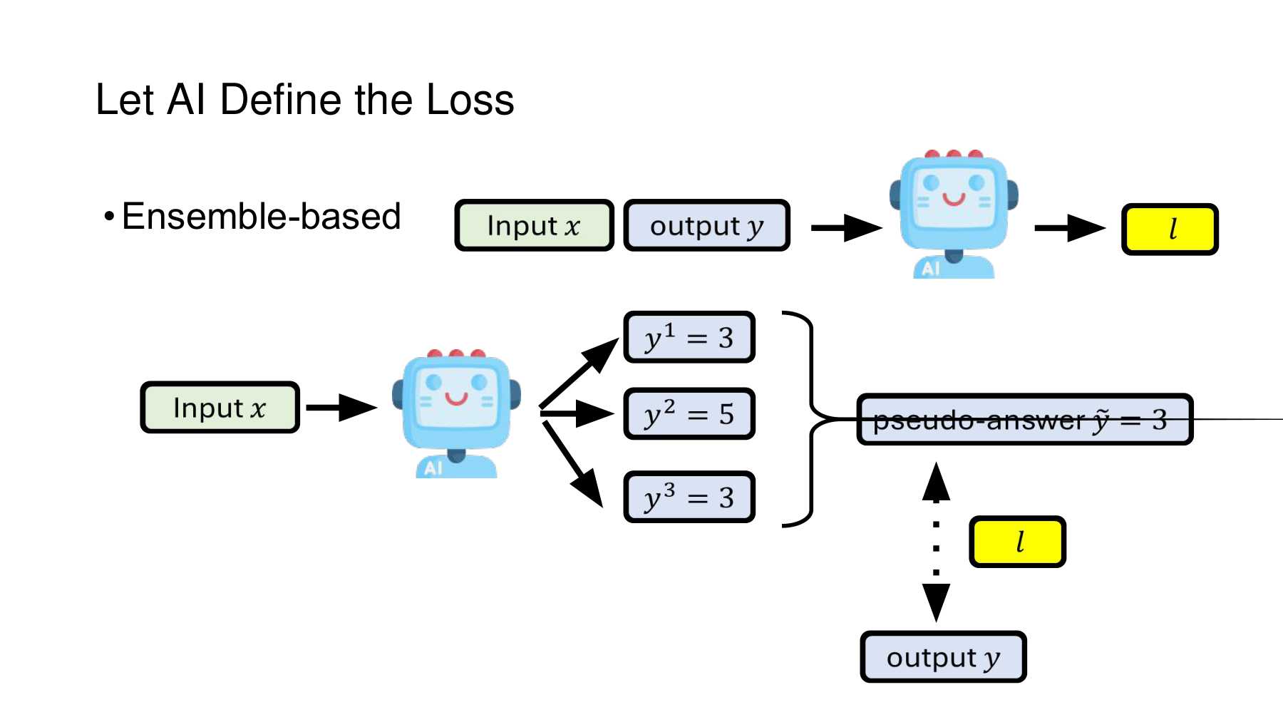
The slide collects 3, 5, and 3 for the same question and selects 3 as the representative answer. This ensemble-based approach uses agreement among outputs in place of an external answer. The ensemble need not comprise three distinct models. Repeated sampling from one model can produce multiple answers.
Suppose an extraction function obtains the final answer from each response. Across samples, the frequency of answer and the majority answer can be written as follows.
With 3, 5, and 3, the sample proportion for answer 3 is 2/3. We know that two of these three samples ended in 3. Interpreting 2/3 as the probability that 3 is correct requires an additional probability model and validation.
#Further reading A — What does self-consistency change?
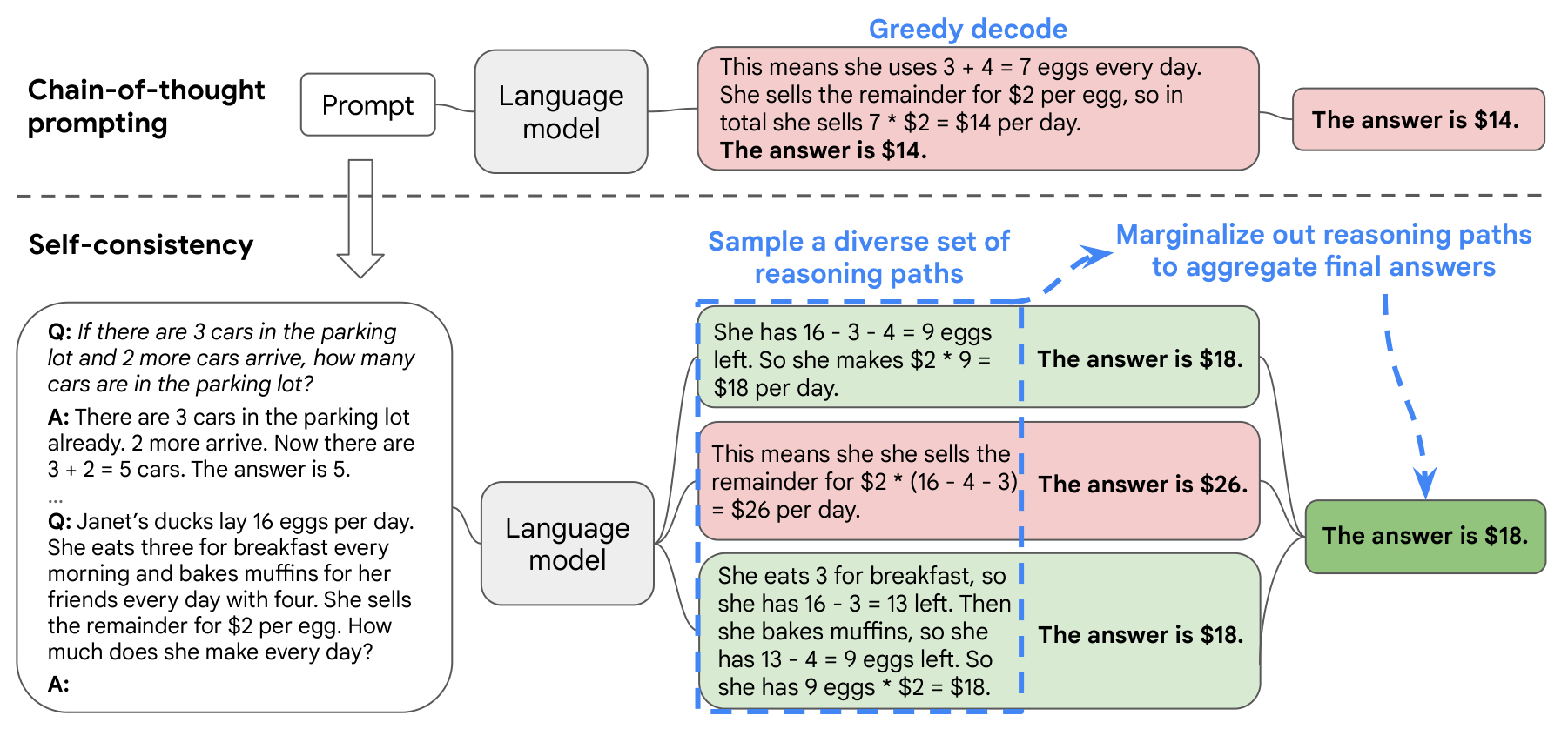
Wang and colleagues’ Self-Consistency Improves Chain of Thought Reasoning in Language Models samples multiple reasoning paths and aggregates their final answers. Figure 1 compares taking a single greedy path with collecting answers reached across paths. Original paper, Figure 1, PDF page 2, and section 2
The figure calls for sampling distinct reasoning paths, extracting final answers in a comparable form, and using their agreement. Simply writing three lengthy explanations does not guarantee improvement. In the original paper, self-consistency is an inference-time decoding and aggregation strategy. Aggregation alone does not train network weights. Sections 2–3
The lecture relates the idea to learning signals more broadly. The aggregate answer can become a pseudo-label for training. Adding a pseudo-label training stage lets the selected answer serve as a target as follows.
Returning 3 during inference differs from increasing the probability of generating 3 through subsequent training. Training may reinforce the error if the pseudo-label is wrong. Measure the quality of aggregation and generalization after training separately.
#What counts as the same answer?
Counting “3”, “3.0”, and “the answer is 3” as distinct strings splits equivalent answers. Ignoring units and merging “3 m” with “3 cm” combines different answers. Fractions, rounding, option formats, and code execution results make extraction and normalization substantive parts of the procedure.
Ties need a rule too. Will we pick an arbitrary label, draw more samples, or exclude the example? The choice changes both the additional compute and the distribution of training data.
#More samples can still share the same misunderstanding
Suppose the model misreads a condition and produces the same wrong answer nine times out of ten. More samples may establish more reliably that the wrong answer is the majority. Aggregation can reduce sampling variation, but it does not automatically correct a shared false assumption.
Even with independent random numbers, all calls share the same model’s knowledge and biases. Independent draws from one distribution differ from independent evidence of correctness. Diverse paths, computation tools, and new evidence can change what agreement means.
#Slide 29 — Entropy measures uncertainty, without access to the correct answer
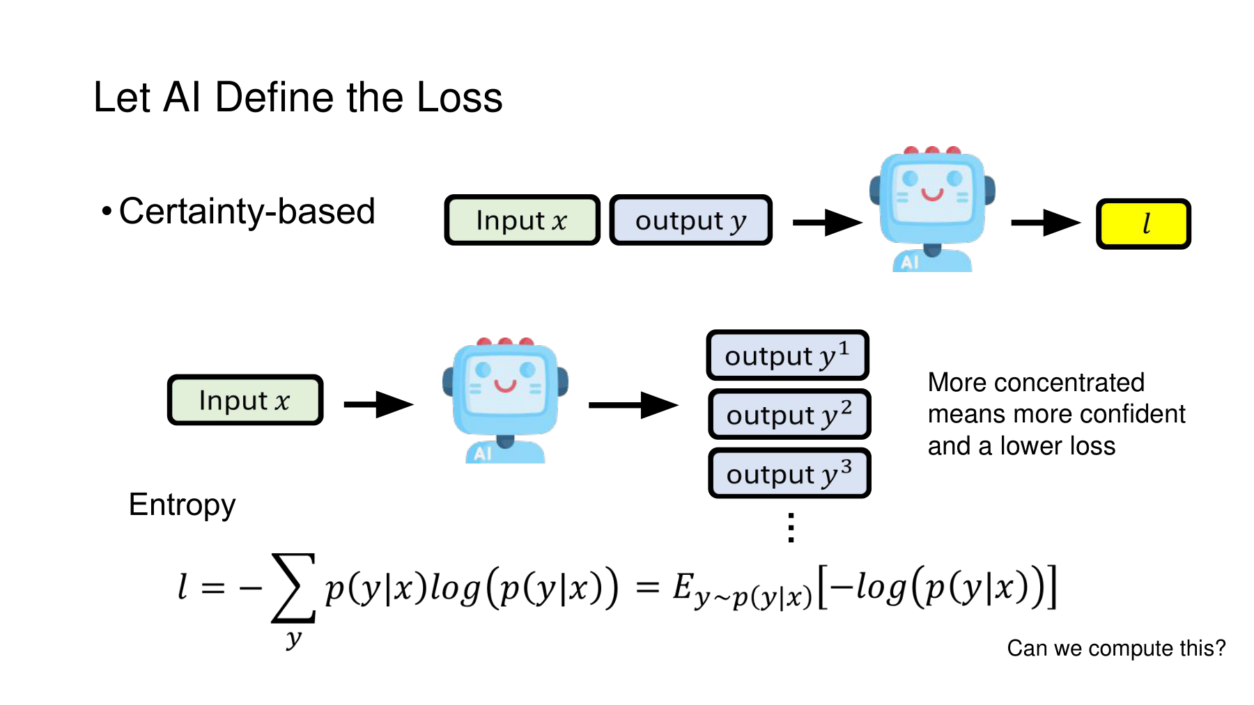
We now inspect output probabilities directly, instead of asking for a score or counting answer strings. The slide interprets greater concentration as greater confidence and connects concentration to a loss. Entropy measures this property.
#It matters which answer receives the probability mass
Start with a finite classification problem. This is Shannon entropy with natural logarithms. The unit is the nat, and a zero-probability term takes its limiting value of zero.
With equal probabilities on three answers, the model favors none. Placing most probability on one answer makes the distribution sharper and lowers entropy.
Whether the answer receiving 0.8 in the second distribution is correct does not appear in the entropy expression. Permuting the answers while keeping the same probability values leaves entropy unchanged.
If the first distribution gives A its highest probability and the second favors B, their most likely answers differ. When B is correct, the second gets it right and the first gets it wrong. Entropy alone cannot reveal that difference.
#A direct calculation — Greater confidence in a worse prediction
Here is an illustrative example with B as the correct answer. Probabilities are ordered A, B, C. The last column gives the negative logarithm of the probability of B, the cross-entropy loss computed when the ground truth is known.
| Distribution | Most likely answer | Entropy | Probability of correct answer B | Ground-truth loss |
|---|---|---|---|---|
| (0.8, 0.1, 0.1) | A: incorrect | 0.6390 | 0.10 | 2.3026 |
| (0.98, 0.01, 0.01) | A: incorrect | 0.1119 | 0.01 | 4.6052 |
| (0.1, 0.8, 0.1) | B: correct | 0.6390 | 0.80 | 0.2231 |
Moving from the first row to the second lowers entropy. But the probability of B falls from 0.1 to 0.01, increasing the ground-truth loss. Both predictions are wrong. Only confidence in the incorrect answer increased.
This is a counterexample to the claim that lower entropy guarantees higher accuracy. It does not imply entropy minimization always fails. Assess gains using experimental evidence and conditions including base-model ability, data distribution, adapted parameters, and training procedure. This distinction is essential for the studies on slide 30. Tent, section 3 · LLM entropy minimization, section 5
#“Can we calculate it?” — Which output space is involved?
The bottom of the slide writes output entropy as a sum and an expectation and asks whether it is computable. In finite classification, access to every class probability allows direct summation. When the output of a language model denotes an entire completed answer, enumerating all sentences becomes a different computational problem.
Even short sentences combine multiple tokens. The possible sequence count grows rapidly with length. At a fixed prefix, in contrast, model logits determine the next-token vocabulary distribution. Entropy of the whole sentence and entropy of one next-token distribution are distinct.
For a fixed length, the entropy chain rule gives the following expression. Real implementations handling stop tokens and variable lengths require corresponding definitions.
Sum next-token entropies across positions while also averaging over the prefixes that can reach each position. Token entropies along a sampled path can help estimate this expectation, but one path’s value is not an exact sum over every possible path. Summing or averaging by length also changes the learning signal. The LLM entropy minimization paper distinguishes token-level and trajectory-level estimation and objectives. Published paper, sections 2–3
Distinguish a third quantity. For answers 3, 5, and 3 on slide 28, the entropy of the empirical answer frequencies is
This quantity depends on extraction, normalization, and sample count. It does not directly calculate the full vocabulary distribution or the distribution over all possible sentences. Calling all three “model entropy” can conceal comparisons of different quantities.
| Quantity measured | Information used | Qualification |
|---|---|---|
| Distribution over complete answers | Probabilities of possible answers | Summing over the entire output space is difficult |
| Next-token distribution at a given context | Vocabulary logits and probabilities | Specify the context, length, and aggregation method |
| Answer frequencies extracted from samples | Multiple responses and answer normalization rules | Values depend on sample size and extraction |
#Slide 30 — What actually changes in images, speech, and language?
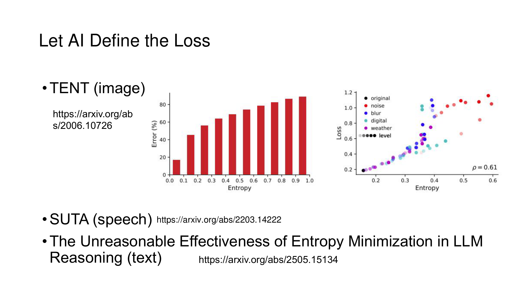
The slide connects Tent for images, SUTA for speech, and entropy minimization in language models. Although all reduce entropy, their models, update targets, and input conditions differ. To interpret separate experiments, ask which distribution’s entropy is reduced with respect to which parameters before attempting any comparison of scores.
SUTA’s methods and settings appear in the arXiv paper and the Interspeech 2022 paper.
#Further reading B — Tent adapts at test time using prediction entropy
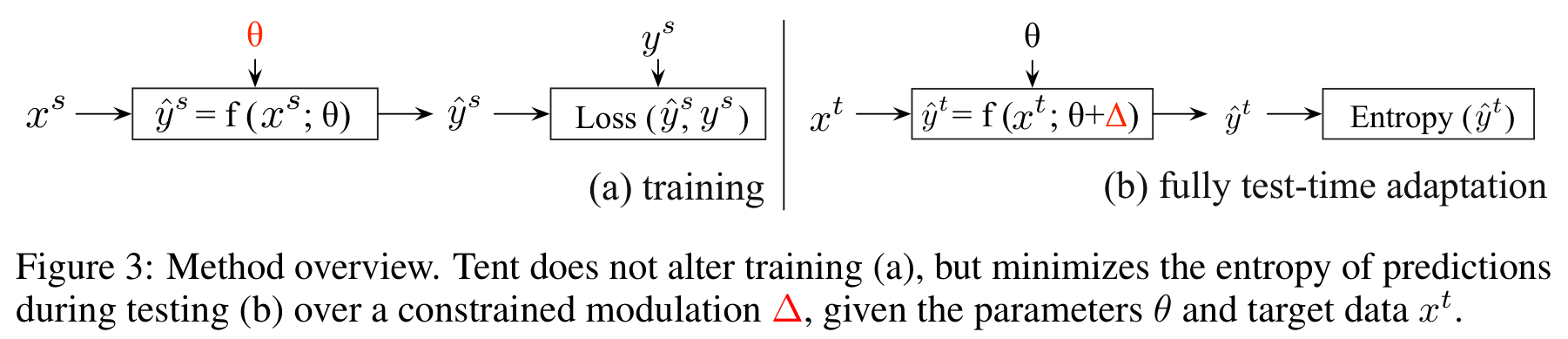
Tent adapts at test time without target labels to inputs whose distribution differs from training. Figure 3 places supervised training with ground-truth labels alongside adaptation using prediction entropy. Original paper, Figure 3, PDF page 3
Tent adjusts limited degrees of freedom for the current inputs. It re-estimates normalization statistics and updates channel-wise affine parameters in normalization layers for the entropy objective. This differs from unrestricted training of all network weights. Section 3, Algorithm 1
For example, test images may be blurrier or noisier than training images. The aim is to adapt to the change while retaining the base classifier’s structure. In this illustration, new test inputs and their distribution contribute information. Absence of ground-truth labels does not mean the system receives no external information.
The Tent graph on slide 30 shows how entropy and error relate in the reported setting. It does not establish a mathematical guarantee that low entropy means correctness for all inputs and models. The slide 29 counterexample rules out a universal guarantee, while Tent tests gains for a specific procedure under specified conditions.
#Further reading C — SUTA: Does the same equation suffice for recognizing a single utterance?
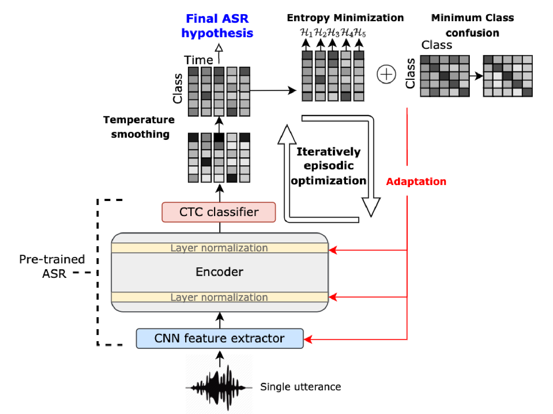
SUTA studies test-time adaptation of speech recognition using a single utterance. At left, the diagram separates the largely frozen model from parameters to adapt. At right, it combines temperature smoothing, entropy minimization, and minimum class confusion. Lin, Li, and Lee, Interspeech 2022, Figure 1, PDF page 1
In speech-recognition CTC outputs, many frames assign high probability to the blank token, which emits no character. Sharpening every distribution unconditionally could strengthen blank predictions instead of meaningful character distinctions. The paper excludes frames whose most likely token is blank from the entropy calculation and adds a class-confusion objective. Sections 2.2.1–2.2.4
Temperature smoothing first makes probabilities less extreme to manage the optimization signal. Training to increase confidence and smoothing the distribution used for the calculation operate at different levels. The name “entropy minimization” does not imply every step sharpens a distribution.
In the paper’s basic experimental setup, layer normalization and the feature extractor are adapted. Each utterance starts from the original model weights. A fixed number of adaptation steps yields the final recognition for that utterance. This differs from accumulating updates indefinitely across utterances. Algorithm 1, section 3.4
Simply applying Tent’s entropy equation to a speech model does not reproduce SUTA. The output structure, blank tokens, adapted components, combination of objectives, and reset rule all matter.
#Language models — EM-FT, EM-RL, and EM-INF are different operations
Agarwal and colleagues’ The Unreasonable Effectiveness of Entropy Minimization in LLM Reasoning applies entropy minimization to both post-training and inference. It distinguishes three methods. Published paper, sections 2–4
| Method | What changes directly | How entropy is used | Updates model weights? |
|---|---|---|---|
| EM-FT | Model parameters | Differentiate and minimize token-level entropy on self-generated outputs | Yes |
| EM-RL | Generative-policy parameters | Use negative entropy as a reward for reinforcement learning | Yes |
| EM-INF | Inference-time logits | Optimize logits during decoding to reduce entropy | No |
EM-FT can resemble supervised fine-tuning on correct sentences, but its objective differs. Instead of minimizing negative log probability of ground-truth tokens, it directly uses output entropy in model-generated contexts. The experiment asks whether existing abilities can be used more consistently without learning from external correct answers. Section 3.1
EM-RL uses negative entropy as a reward. The paper distinguishes forms based on the log probability of an entire trajectory from those using token-level distributions. These calculations yield different updates. The reward is not a ground-truth correctness check. Distinguish higher reward from improvement on a separate evaluation with correct answers. Section 3.2, Table 1
EM-INF draws an especially clear boundary. It optimizes logits during inference and leaves model weights fixed. Even if an answer improves, that alone does not show new knowledge was stored in weights. The distinction from Part 1 between improving output production and training parameters applies here. Section 4
#Further reading D — Conditions hidden by looking only at favorable results
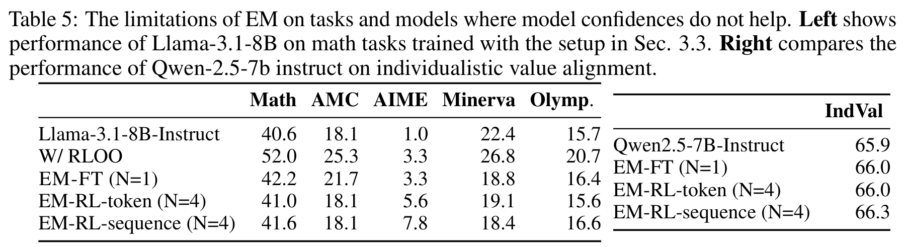
Table 5 of the same paper explores limitations. At left are math tasks using Llama-3.1-8B-Instruct. At right is a personalized value-judgment task using Qwen-2.5-7B-Instruct. The table does not support consistent improvement across all models. Table 5, PDF page 9, and section 5
In the Minerva column, base Llama-3.1-8B-Instruct scores 22.4 and EM-FT scores 18.8, though some other columns improve. On IndVal, the three entropy methods score 66.0, 66.0, and 66.3 against a baseline of 65.9. These small differences alone cannot establish reliable gains. The table provides no confidence intervals from which to judge their statistical significance.
The authors emphasize the base model’s initial reasoning ability and whether its confidence suits the task. Concentration can help an existing skill express itself more consistently, but can also strengthen incorrect knowledge or prior biases mismatched to the task. This is the authors’ interpretation of their experiments, and a model name alone cannot predict success or failure on every new task. Sections 5–6
#Reinforcement learning sometimes increases entropy. Is that a contradiction?
RL intended to preserve exploration can add an entropy bonus to prevent actions from collapsing too early onto one choice. Its direction is opposite to entropy minimization, but different objectives and training stages can require different signals.
Exploration matters when useful actions in a new environment have yet to be found. In a pretrained model with useful capabilities already present, concentrating probabilities can help elicit them more consistently under some conditions. Neither direction is universally correct. Ask first which distribution is being adjusted, for what objective, and with which base model. The LLM paper also distinguishes prior entropy regularization from its standalone minimization objective. Sections 2–3
#What to record when comparing the three signals
| Signal | What it directly measures | Common misinterpretation | What to check separately |
|---|---|---|---|
| Verbal self-evaluation | Rating or affirmative response under an evaluation prompt | A high score or Yes probability equals probability of correctness | Relationship with ground truth and sensitivity to criteria and wording |
| Agreement across responses | Sample frequency of extracted answers | A repeated wrong answer becomes correct by majority vote | Normalization, shared errors, sample count, compute budget |
| Entropy | Uncertainty or concentration of a distribution | A sharper distribution is more accurate | Independent accuracy, base-model capability, adapted parameters and conditions |
Use the table to validate an implementation. Record at least actual task performance and the change in the proxy signal separately. A rise in self-evaluation scores without greater accuracy differs from selecting a better answer using a larger token budget.
Specify the test-time adaptation protocol. Does each input reset to the base model, or are prior updates retained? Did labels guide adaptation or configuration selection? Adapting to unlabeled test inputs differs from leakage through choosing a method after seeing test answers. Repeatedly using final comparison labels to choose settings weakens an evaluation’s independence.
Record costs, inputs, and starting-model conditions for each method. Where possible, report variation across seeds and failure cases as well.
#Three questions to check understanding
1. If a model gives the same answer nine out of ten times, does it have a 90% chance of being correct?That is the observed sample frequency of an answer. A systematic misunderstanding could recur. Using the frequency as a probability of correctness requires a separate definition and validation.
2. If entropy falls, must the ground-truth loss fall?No. When B is correct, concentrating more probability on A can lower entropy while increasing B’s negative log probability. The three-class example provides a counterexample.
3. Do Self-Consistency and EM-INF train model weights?Self-Consistency as examined here samples multiple paths and aggregates their answers at inference. EM-INF adjusts inference logits without updating weights. An additional training procedure can use the results, but distinguish it from each method’s original operation.
Across these five slides, signals can be constructed without ground truth, but their meaning and actual improvement require separate validation. The next section covers slides 31–35, on learning from self-evaluation signals and changes at test time. Next: Self-Improving AI 07 — When Should Self-Training Stop, and When Should a Model Adapt?.
#Original sources for further reading
| Source | Version and location | Topic |
|---|---|---|
| NTU Self-Improving | May 8, 2026 lecture, PDF pages 26–30 | Main lecture and three evaluation signals |
| Self-Consistency | arXiv v4 / ICLR 2023, Figure 1 on PDF page 2 | Multiple reasoning paths and aggregation of final answers |
| Tent | arXiv v3, March 18, 2021 / ICLR 2021, Figure 3 on PDF page 3 | Prediction entropy and normalization parameter adaptation |
| SUTA | Interspeech 2022, printed pages 2198–2202, Figure 1 on PDF page 1 | Single-utterance adaptation of CTC speech recognition |
| Entropy Minimization in LLM Reasoning | Published NeurIPS 2025 paper, sections 2–5, Table 5 on PDF page 9 | EM-FT, EM-RL, EM-INF, and dependence on the base model |