The same language model can become a different agent depending on the information it receives, the tools it uses, and what it does after failure.
Part 14 examined how a proposer, solver, and verifier generate learning problems and rewards. That loop still contains human-designed problem instructions, execution environments, and answer checks. Here the question shifts from training the model’s weights to improving the way the model is used.
A harness is the system surrounding a model that assembles its inputs, connects tools, and controls execution order. An AI can change agent behavior by editing that code or rewriting instructions. Producing a revision, however, does not establish that the revised system works better. Following slides 6–10 of the second lecture, this article examines both what can change in the harness and what evidence should guide selection.
Worked examples Context budget · Prompt–weight interaction · Selection bias
Video locations by slide
The links identify remarks on each topic. The timestamp for the prompt examples on slide 6 refers to the proposer’s and solver’s roles discussed in the previous part. It does not locate a verbatim reading of the prompts or the exact slide transition.
| Slide | Video | Topic |
|---|---|---|
| Second half, 6 | From 4:45 | Review of the proposer and solver, overlapping the previous part |
| Second half, 7 | From 5:15 | The harness and language model that make up an agent |
| Second half, 8 | From 5:36 | Changing the target of improvement from model to harness |
| Second half, 9 | From 5:48 | Harness updates, evaluation, and the question mark on gradient descent |
| Second half, 10 | From 7:07 | How an AI proposes harness revisions |
#Second half, slide 6 — Self-learning has a designed starting point
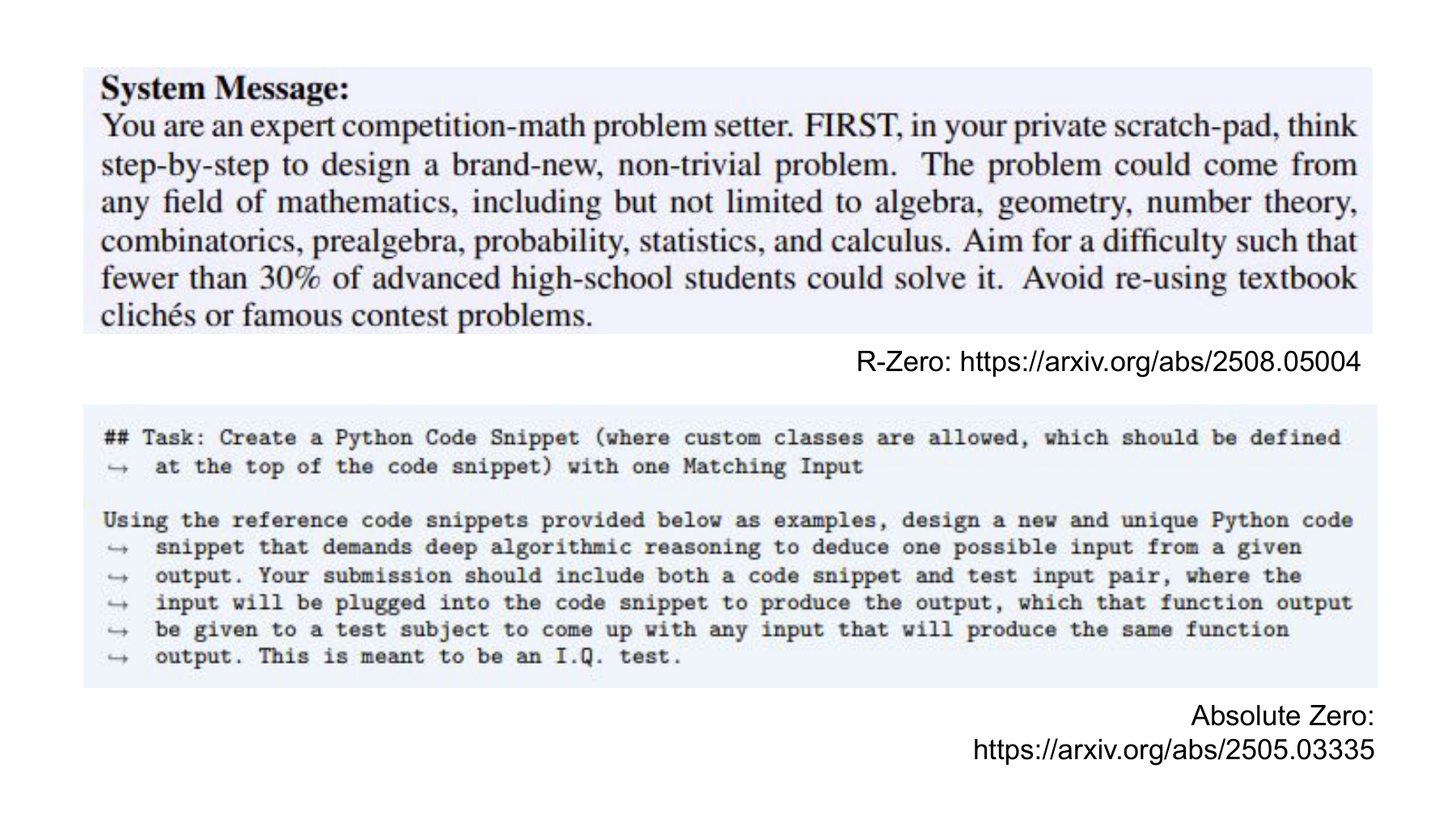
The slide’s two examples show where the earlier self-learning systems begin. R-Zero’s prompt specifies the role and type of math problem to generate. Absolute Zero’s prompt specifies how code and inputs relate. Even when a model generates new problems, what it should generate, the required format, and the verification environment are already structured.
Distinguish an objective written in an instruction from a measured result. Asking for a difficult problem or targeting an accuracy rate gives the proposer a direction. It does not establish the problem’s difficulty for real people. Likewise, requesting an output format does not guarantee compliance on every run.
This distinction leads to harness improvement. Changing a proposer prompt can change the kinds of problems generated. Adding code that filters invalid formats can change the data passed downstream. Both affect system behavior without updating model weights at that point. This connects the self-learning loop to harness design.
After changing a proposer instruction, read the raw outputs alongside the execution log. Suppose ten requests produce seven outputs the parser can read and five of those pass the executable task checks. The fraction valid among parsed outputs is 5/7. The number of valid tasks obtained per request is 5/10. If a parser fix recovers the three previously unreadable outputs, check the validity of those three. The parser now accepts more outputs. Running the checks tells us how many additional tasks are fit to train on.
#Second half, slide 7 — An agent combines a model and a harness
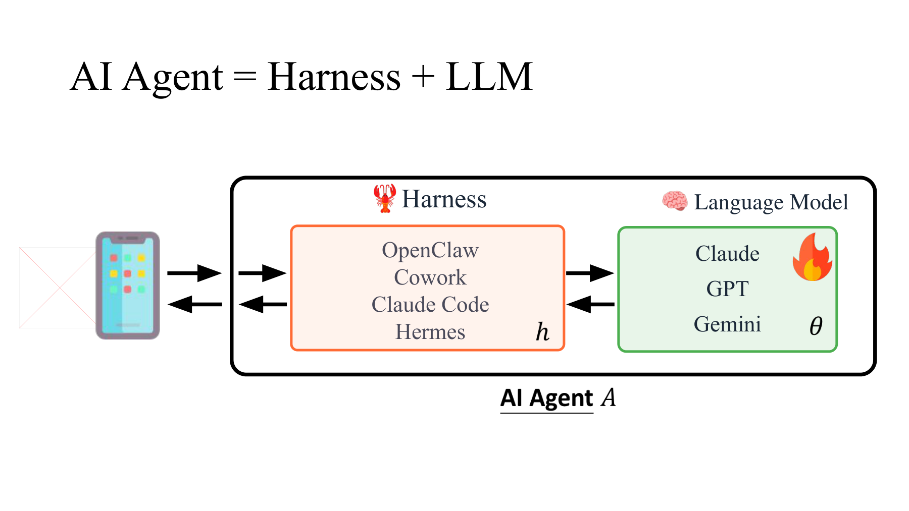
“Harness + LLM” describes system composition. A language model receives context and produces a response or a tool call. The harness decides which context to provide, how to execute a generated call, and how to insert its results into the next input. Lecture at 5:15
Following the slide, use θ for the model parameters and lowercase h for the harness. Then the agent can be written as:
| Symbol | Meaning | Example change |
|---|---|---|
| θ | Learned weights of the language model | Fine-tuning or reinforcement learning updates internal parameters |
| h | Configuration that calls the model and connects it to the environment | Instructions, tool specifications, output parsers, execution order, retry and memory rules |
| H_info | Human-provided objectives, data, and evaluation information | Requirements, reference examples, grading rules |
Capital H in Part 14 denoted human-provided information. Lowercase h here denotes the harness. We retain H_info for the former. The categories need not be physically separate files. A human-written objective can appear in the harness’s system instructions. Distinguish the configuration open to optimization from the evidence used to evaluate it.
Consider two search-tool interfaces. One returns an entire long document, and the other supplies its location, the relevant paragraph, and its source. With identical model weights, the next decision receives different information. After a tool call fails, the harness also decides whether to repeat the request or expose the error type so the model can revise the arguments.
#A related CMU lecture — How memory is retained is part of the harness
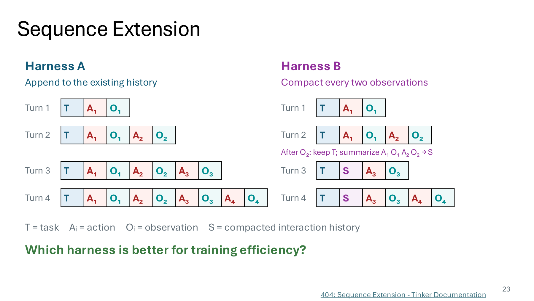
CMU’s “Reinforcement Learning Systems” compares two harnesses. A on the left keeps appending actions A and observations O to task T. B on the right replaces earlier interactions with summary S after two observations. The difference is what the next model call sees. CMU, slides 19–20
Imagine a code-editing agent reading a file and then running a test. A supplies the full code excerpt and error log on the next call. B might summarize them as “Empty input raised an exception in parse_input.” In this illustration, a shorter input could omit the reproduction conditions or exact line number, making the repair harder. A long history filled with irrelevant material could also make the important error harder to find.
The slide’s closing question concerns training efficiency. Slide 20 shows A’s trajectory as one continuous training example. For B, the records before and after summarization become separate examples, each including task T. A shorter inference input therefore does not establish lower total compute. Examine inference context length separately from the computation repeated when training on those records later. CMU, slide 20
Possible interventions include when to summarize, which error details to preserve, and how to format tool responses. All are part of h. Compare success rate and token usage, and also investigate failures caused by details lost in summarization. Even with fixed θ, the rules for presenting observations can change subsequent behavior.
#Can a sixth tool record fit in the same context window?
Give harnesses A and B in the CMU diagram an illustrative token budget. Each call has a 4,096-token context window. Instructions, the current request, and tool definitions use 700 tokens. Reserve 600 for the output. Assume a tool call and its return together occupy exactly 480 tokens. The space left for history is the full window minus the fixed input and the output reservation.
A can fit five full records. Six take 2,880 tokens, exceeding the history budget by 84. If B replaces the first four with a 200-token note and keeps the two most recent records intact, its history uses 1,160. The next input saves 1,720 tokens. What information did it lose? Suppose an inspection record specified a tolerance of 0.2 mm and the note retained only “dimensions checked.” The next request cannot recompute the bounds. Require the summary to preserve units and tolerances, then rerun the same task to test that failure. These figures budget the input for one call under a fixed-length assumption. Count the cost of generating the summary and of subsequent training separately. CMU Lecture 12, pp. 19–20
#Second half, slide 8 — The flame moves from θ to h
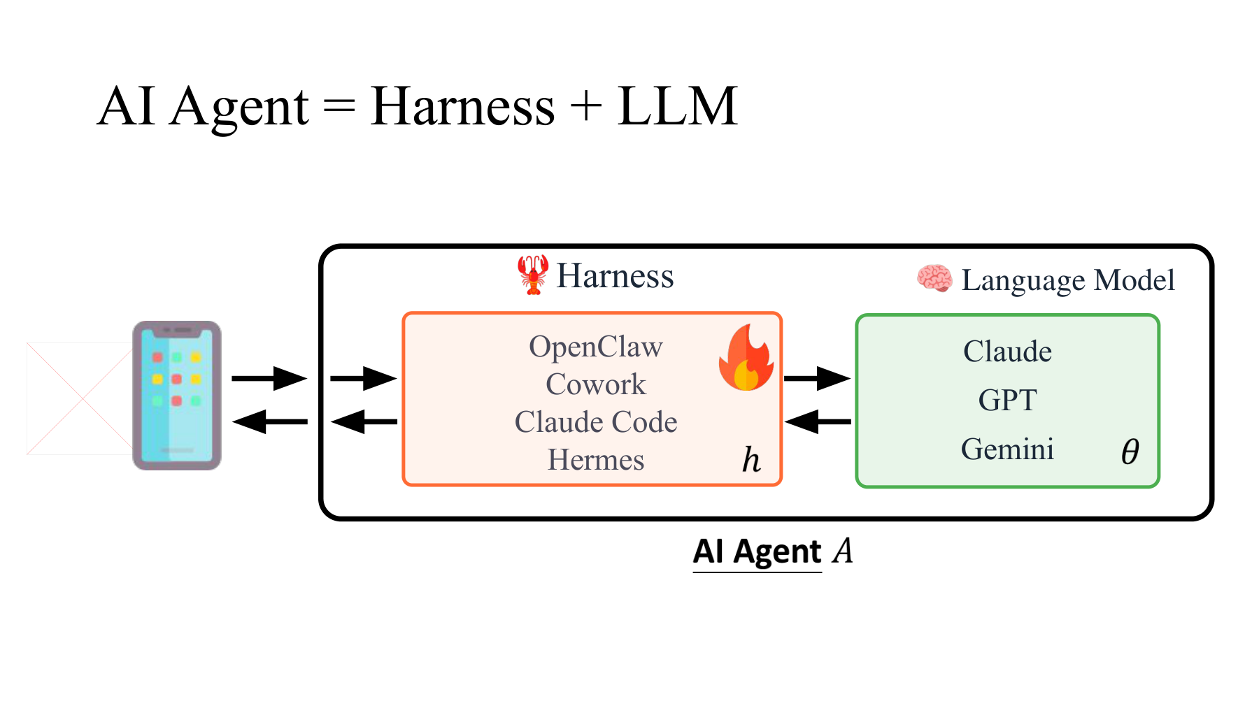
The principal difference between slides 7 and 8 is the position of the flame. The marker moves from the model to the harness. The two changes can be written side by side:
In the second case, the system changes without retraining the model. Generating one longer answer differs from revising a harness that can be reused across tasks. Preserve revised instructions, code, or memory rules in a form that can run again, so the configurations can be compared.
Fixing θ alone does not complete the comparison. Differences in model version, tool access, starting data, execution budget, or success criteria can mix several effects. If h′ uses twice as many model calls as h, the observed difference is the effect of the system including the extra calls. A costlier design may be worthwhile, but an efficiency claim requires a matched-budget comparison.
#If the weights and the instructions both changed, which contributed?
Suppose the original model and instructions solved 70 of 100 tasks, and the configuration that changed both solved 86. Those two numbers cannot tell us how many of the 16 extra successes came from the harness. Run the two intermediate combinations on the same tasks with the same tools and call budget. Here are hypothetical success counts.
| Same 100 tasks | Original instruction h₀ | New instruction h₁ |
|---|---|---|
| Original weights θ₀ | 70 | 80 |
| New weights θ₁ | 85 | 86 |
Read across a row to change the instruction while holding the weights fixed. The gain is 10 percentage points with the original model and 1 point with the new one. The difference of −9 points means the new instruction adds nine fewer points with the new model on this evaluation. It still increases the score in both rows. BetterTogether alternates weight and prompt optimization, giving a concrete reason to reevaluate instructions after changing the underlying model. The table illustrates that dependency. Generalization beyond these 100 tasks would require evaluation data excluded from candidate selection and repeated runs. BetterTogether, EMNLP 2024
#A related NAIRR lecture — Distinguishing a reflective note from a harness update
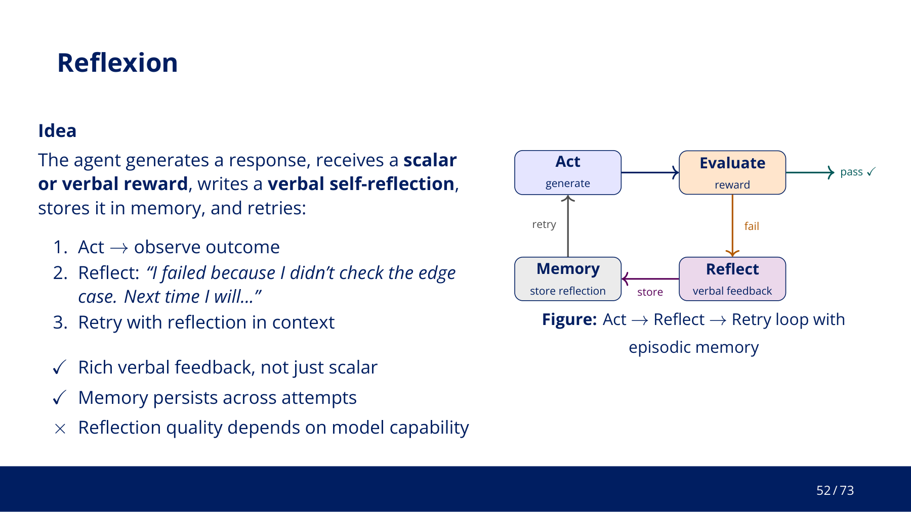
NAIRR’s “Training-Free Alignment of LLMs” distinguishes three intervention points. Before generation, change the prompt. During generation, adjust token selection. After generation, inspect, filter, or revise the completed response. The tutorial calls the last approach response engineering. Slides 38–40 · Lecture, 2:07:29–2:09:28
Slide 52 shows Reflexion. The agent acts, receives an evaluation, describes the cause of failure in words, and puts that description into the next trial’s context. The lecture follows action → evaluation → reflection → memory → retry. The model’s capabilities limit the quality of the reflection. Writing an explanation does not establish that the diagnosis is correct. Lecture, 2:21:42–2:22:53
Mapping this example onto θ and h requires distinguishing a run that appends one reflection under an existing rule from an experiment that changes the rule for producing or using reflections.
| Change | What changes directly | Interpretation here |
|---|---|---|
| After a failure, add “Check empty inputs” to the next attempt | Contents of runtime memory | A fixed harness updates state according to its rules |
| Change when to reflect, what to record, or when to retrieve it | Memory creation and use rules | A candidate harness h′ reusable across runs |
| Fine-tune on records of successes and failures | Model parameters | An update to θ |
The first system can use earlier experience to improve a later attempt. If the target h is defined as the rule for creating and using memory, changing the note’s contents alone does not show that the harness code improved. Define the variables and controls before comparing runs.
For example, one harness could store every reflection after every failure. Another could retain only causes confirmed by tests and prune stale notes. These are competing memory policies. Compare their success rates and costs on new tasks. The NAIRR lecture also describes the latency, cost, nontermination, and debugging difficulties that repeated processing can introduce. Slides 50–52 · Lecture, 2:19:42–2:21:39
#Second half, slide 9 — Can gradient descent be applied directly to a harness?
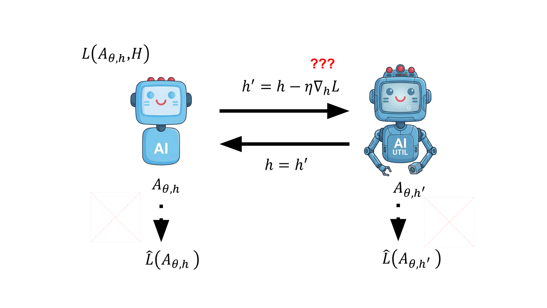
The lecturer adds harness h to the earlier diagram of learning. Let L denote the objective or feedback the system uses and L̂ the evaluation that checks the result. Smaller values of both losses are better.
The slide then presents a familiar-looking gradient descent expression with three red question marks. The expression poses a question. It is not an update rule ready to execute on an arbitrary harness.
Gradient descent requires a variable with a defined continuous variation. Changes such as adding a verification step after search, retrying only on failure, or clarifying a tool description have no given real-valued coordinate to differentiate or subtract. Harness code and strings cannot simply be treated as model weights. Lecture, 5:48–7:07
Individual numeric parameters in a harness can be optimized continuously, and differentiable representations can be designed. Neither makes the expression automatically valid for an arbitrary combination of prompts, branches, and tool connections. What is needed is a procedure to generate revisions and decide which to retain from their results.
#Worked example 1 — Pairing results to see which tasks improved
Consider a hypothetical experiment comparing two harnesses with a fixed model. Both run once on the same 100 tasks, with matched initial states, execution budgets, and success criteria. Suppose the paired outcomes are:
| Outcome on the same task | Number of tasks |
|---|---|
| Both h and h′ succeeded | 60 |
| Only h succeeded | 10 |
| Only h′ succeeded | 20 |
| Both failed | 10 |
Write s_i(h)∈1 for success on task i. The mean success rates and their difference are calculated below. From here we use success rate S, where larger is better.
The new harness scores 10 percentage points higher on these runs. It gained 20 successes and lost 10 others, a pattern that comparing two averages can hide. Reviewing the failures suggests hypotheses about which problem types the revision helped or hurt.
This summarizes the 100 observed tasks. It neither guarantees a 10-point gain on new tasks nor establishes statistical significance. If generation or environment behavior is stochastic, repeat each task. Reset state before each run to keep edited files or conversation history from leaking into another condition.
#Second half, slide 10 — AI proposes revisions and execution results guide selection
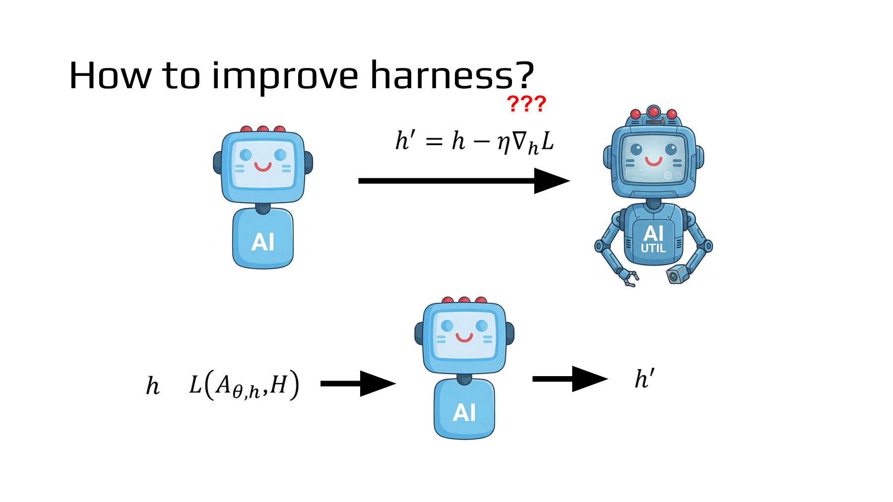
Slide 10 replaces the question marks with a different operation. Give an AI the current harness and signals from its runs, and ask it to propose a new harness. A model that handles language and code can revise instructions, choose examples, add steps, or change branch conditions. This is a different operation from differentiating strings numerically. Lecture at 7:07
For a concrete design, let F_dev contain development scores, failure types, tool responses, and differences from expected results. Write q_φ for the candidate generator. The model proposing revisions may be the target model or a separate fixed model. φ denotes the generator’s parameters, without implying any weight update during proposal.
Check that each candidate runs, compare candidates on development tasks, and select the next configuration. For instance, let C_t be the valid candidates and include the original configuration in the comparison. The following is one possible selection rule. Different studies may use different procedures.
Including the original configuration lets the search reject lower-scoring alternatives under the same development evaluation. This protects only the observed development score. Stochastic variation and overfitting to development tasks can still reduce true expected performance. Tasks repeatedly used for selection cannot also serve as an independent final evaluation.
The lecturer also notes that an AI’s internal criterion may differ from the human’s final objective. A persuasive explanation of a proposed edit does not establish a reduction in L̂. Lecture at 7:40
#A related MIT lecture — Generating candidates and choosing among them
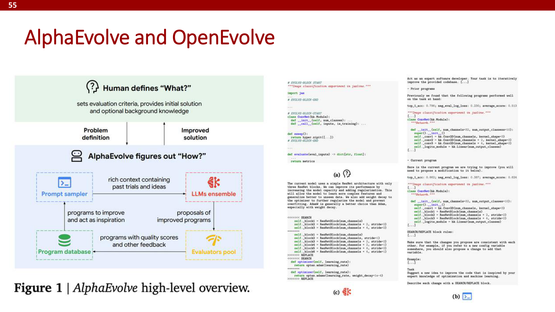
Slide 55 of MIT’s “Self-evolving AI” lecture describes AlphaEvolve and OpenEvolve. The top of the left diagram shows the human-defined evaluation criterion, initial solution, and background knowledge. Below, stored programs are sampled for a prompt, a language model proposes a revision, and an evaluator scores its execution. The programs and evaluation records inform future proposals. MIT, slides 53–55 · Official lecture video
Beside NTU slide 10, the diagram shows which steps follow “AI writes new code.” A code proposer, execution environment, evaluator, and archive of previous attempts each have a role. Errors and low scores from failed programs can inform future revisions. Reading those records alone cannot guarantee a correct fix.
AlphaEvolve changes a program for solving a specified problem. Its diagram is not evidence that the entire harness rewrites itself. The connection here is generating programs and selecting among them by execution results. Restrict search to harness prompts, tool-call code, or execution order, and it can take the form of the search over h described above. AFlow, discussed later, makes this connection concrete for workflows.
The evaluator matters. If runtime alone determines reward for a file-processing program, one that skips inputs may score highly for speed. This illustrative example explains the criterion rather than reporting a lecture result. Verify output correctness and input coverage before comparing runtimes. For harness revisions, also decide in advance how to treat hidden failures and successes achieved with extra calls.
Alongside candidate scores, record the evaluator version, execution environment, inputs, and costs. The next example shows how changing just a cost constraint can change the selected harness.
#How often will a search over ten candidates turn up a perfect development score?
The selection rule on page 10 retains the highest development score. A lucky candidate can win even when all candidates are equally capable. Suppose the development set has four tasks. Every candidate succeeds on every task with probability one half. Assume the outcomes are independent across tasks and candidates. First compute the probability that one candidate gets a perfect score. Then take the complement of the probability that all ten miss it.
A candidate fixed in advance has a 6.25% chance of getting all four right. The chance that the best of ten gets all four is about 47.6%. Whichever candidate wins, its success probability on a fresh independent task in this example remains 50%. Cawley and Talbot explain how optimizing a selection criterion estimated on a finite sample can fit its random fluctuations. Actual harnesses often share a base model and its errors. If their perfect-score events coincide exactly, the chance of a perfect score remains 6.25% even with ten candidates. The 47.6% figure depends on independence. This is why we select one candidate on development tasks, then evaluate the selected harness on held-out tasks. Cawley and Talbot, JMLR 2010
#Worked example 2 — The highest success rate and the best candidate within budget
This separate hypothetical comparison uses the same model and 100 development tasks. Add input and output tokens and average by task. Token usage is the resource measure in this example. It need not equal actual price or latency.
| Harness | Successful tasks | Success rate | Average tokens per task | Total tokens for 100 tasks |
|---|---|---|---|---|
| A | 70 | 70% | 1,000 | 100,000 |
| B | 80 | 80% | 2,000 | 200,000 |
| C | 78 | 78% | 1,500 | 150,000 |
To maximize success rate alone, choose B. If the design must average at most 1,500 tokens per task, B is ineligible and C wins. Write T̄(h) for average tokens and B_tok for the budget. The selection rule is:
C scores eight percentage points above A and uses 50% more tokens. B solves two more tasks than C using 50,000 additional tokens in total. Thus the observed incremental token cost per additional success between B and C is 25,000. This ratio describes these runs. It cannot predict the exact cost of the next additional success.
An average constraint also differs from a per-task limit. If a single slow request matters, inspect maximum token usage or upper latency quantiles. Distinguish the cost of running the chosen harness from the cost of finding it. Let T_search be search tokens, Q the number of tasks after deployment, and T_run the mean execution tokens. Total usage is:
If finding C costs 300,000 tokens, its total through 100 subsequent tasks is 450,000 tokens. Counting only execution yields 150,000. Interpreting optimization efficiency requires stating which costs were counted.
#Supplement A — SWE-agent changes the form of actions and observations
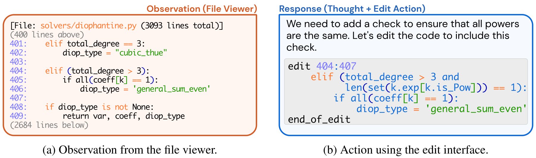
SWE-agent treats the agent–computer interface (ACI) as a joint design problem involving the commands a model uses and feedback from its environment. The viewer shows file location and line numbers, and the editing command refers to those lines. The paper compares interfaces with a fixed base model. Paper, sections 2–3 During development, people analyzed trajectories and performed a grid search over configurations. Paper, section 4, Configuration search
The intervention changes what the model sees and the granularity of its actions, with code-representation weights held fixed. A command convenient for a person may not be the easiest for a model to use. Immediately seeing relevant code and errors after an edit changes the context for selecting the next action.
SWE-agent illustrates concrete harness features that can affect performance. The design study itself does not show that AI automatically invented its harness. The next two examples make automatic revision and selection more explicit.
#Supplement B — DSPy separates a program from its optimization
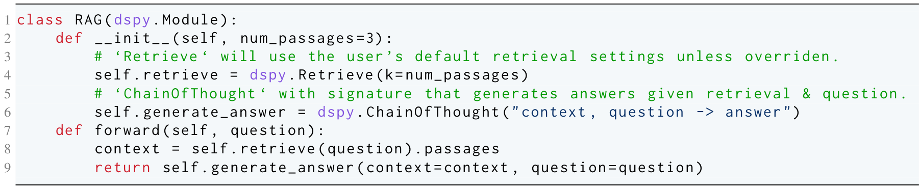
The program takes a question, retrieves documents, and passes the question and retrieved context to the answer module. DSPy distinguishes this program from the procedure that uses data and metrics to optimize it. The original compiler collects useful demonstrations from execution traces and selects candidates to construct module prompts and related settings. Paper, sections 3.3–4
Choosing demonstrations for a fixed-weight model counts as improving h here. DSPy also supports fine-tuning with collected demonstrations, so fixed θ is not a framework-wide requirement. This discussion focuses on optimizing the configuration and demonstrations of a program that calls the same model.
An experimental configuration needs more detail than a model name. Results with the same base model depend on which program was optimized, with which data and metric. Keeping the program, selected examples, and optimizer settings turns “we found a good prompt” into a configuration others can rerun and compare.
#Supplement C — AFlow searches workflows expressed as code
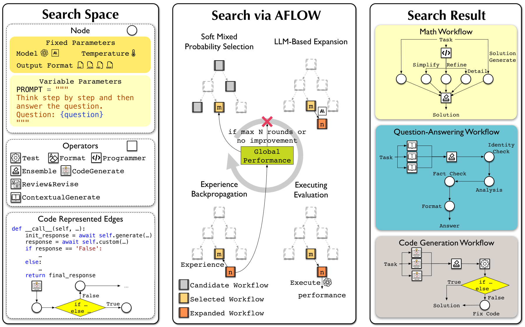
AFlow expresses model calls and their connections as code, then searches workflow candidates with a variant of Monte Carlo tree search (MCTS). Its practical search space fixes the model, temperature, and output format and revises prompts and code-defined connections. Each node in the search tree represents one complete workflow, rather than one model call. Paper, sections 3.2–4
The LLM proposing edits considers earlier changes and results, and the revised workflow is run to obtain a development score. “Experience Backpropagation” in the figure means propagating search records and scores to ancestor candidates. It differs from propagating gradients through a neural network’s θ.
This makes the arrow on slide 10 concrete. Code generation expands the candidate pool, while execution and evaluation guide future choices. The operators, runtime environment, scoring function, and search budget remain specified. A claim of automatic discovery therefore needs an account of the search space and evaluation conditions.
#Supplement D — τ-bench distinguishes succeeding once from succeeding repeatedly
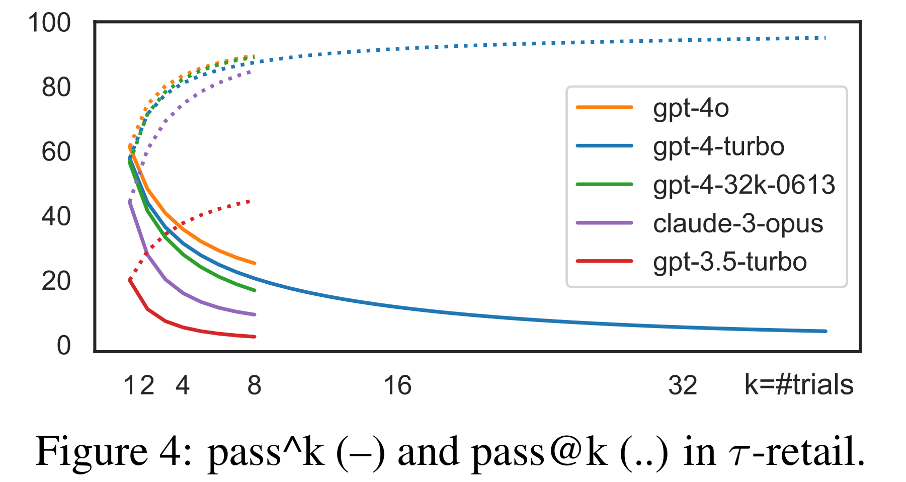
In τ-bench an agent completes tasks through interaction with tools and a simulated user. The figure compares two metrics from the 2024 τ-retail experiments. pass@k asks whether at least one of k attempts succeeds, and pass^k asks whether all k succeed. The figure describes historical experiments rather than current model rankings. Paper, sections 3 and 5
Let p_i be the probability of success on one attempt at task i. Reset the task between runs and assume that, conditional on the task, attempts are independent and identically distributed. The first expression below multiplies the success probability k times. The second subtracts the probability of k failures from 1.
Across tasks, compute these quantities for each task and then average them.
Raising the overall average success probability to the kth power generally gives a different value because tasks vary in difficulty. For k=2 the difference is exact. The variance below measures variation in success probabilities across tasks.
At the same overall average, repeated-run metrics depend on which tasks the system solves consistently and which it repeatedly fails. A high pass^k by itself cannot establish uniform reliability across tasks.
#Worked example 3 — Estimating both metrics from observed success counts
In practice p_i is unknown. Running task i a total of n_i times yields c_i successes. For n_i≥k, τ-bench uses the combinations below. Count all ways to select k runs for a task, then count the selections satisfying each condition. Paper’s estimators
Under the independence and identical-distribution assumptions above, both expressions are unbiased estimators of their target probabilities. A combination is zero if its upper argument is smaller than k. These expressions differ from raising the observed ratio c_i/n_i to the kth power.
Run two hypothetical tasks five times each, resetting between runs. The first succeeds four times and the second twice. Evaluate k=2. There are ten ways to choose two of the five runs for either task.
| Task | Success count | Pairs where both succeed | Pairs where at least one succeeds |
|---|---|---|---|
| First | 4/5 | 6/10 | 10/10 |
| Second | 2/5 | 1/10 | 7/10 |
The same records yield a 60% mean single-run success rate, a 35% estimate for both runs succeeding, and an 85% estimate for at least one success. A task whose successful retry can be recognized and selected calls for a different metric from one that must complete reliably on every request. pass@k alone does not establish that the deployed system can identify the successful response.
Repeated reliability also depends on what counts as success. The τ-bench paper acknowledges that an agent can produce the correct final database and required response yet violate a policy, for example by omitting user consent. pass^k measures repeated success under the stated scoring rule and cannot certify compliance with every policy. Limitations of the reward definition
#How to read claims of harness self-improvement
These five slides build a connected argument. Slide 6 shows the role of predefined direction and output format in generating self-learning problems. Slides 7–8 shift the target from model weights to the harness. Slide 9 asks how that harness can be optimized. Slide 10 introduces an AI that generates candidate revisions.
To evaluate the process, record the revision target, comparison conditions, and selection criterion. Include harness code and instructions, the exact base-model version, initial tool and environment state, development and final evaluation data, repetitions, and execution budgets. Distinguish selection scores from independent evaluation scores. Compare average performance, costs, and failure types to establish where the improvement holds.
AI-generated edits are one important step. Executing them, learning from failures, and selecting the next configuration under comparable conditions complete the research loop. Part 16 starts with slide 11 of the second lecture and focuses on prompt optimization.
Calculations and code
The code calculates paired success differences, budget-constrained candidate selection, combined search and execution tokens, and the combinatorial estimators for pass^k and pass@k. It checks task records against the aggregated table and verifies the estimators by enumerating all eligible groups of attempts. A separate calculation checks unbiasedness by assigning exact probabilities to every outcome in a small Bernoulli experiment. All numerical examples are illustrative and do not rerun the papers’ benchmarks.
#Further reading
| Resource | Relevant topic |
|---|---|
| NTU second lecture · Slides 6–10 | Human-provided information, harnesses and models, and AI-proposed harness revisions |
| SWE-agent: Agent-Computer Interfaces Enable Automated Software Engineering | Fixed-model ACI design and action and observation formats |
| DSPy: Compiling Declarative Language Model Calls into Self-Improving Pipelines | Modular programs and optimization against data and metrics |
| AFlow: Automating Agentic Workflow Generation | Code-defined workflows and search using execution feedback |
| τ-bench: A Benchmark for Tool-Agent-User Interaction in Real-World Domains | Tool and user interaction, success definitions, pass^k, and pass@k |
| CMU RL Systems, slides 19–20 · Official lecture video | Appended versus summarized histories and their representation for training |
| NAIRR, slides 38–40 and 50–52 · Video at 2:07:29 · 2:19:42 · 2:21:42 | Response engineering, repeated evaluation and revision, reflective memory, and cost |
| MIT Self-evolving AI, slides 53–55 · Official lecture video | AlphaEvolve candidate generation, evaluation, and records under human-defined objectives and criteria |