The lights dim above a factory inspection camera. You adjust the vision model on the first frame, and it can pick out the part again. Which model should read the second frame? The recent adjustment could help if the lighting stays the same. If the next frame comes from a brightly lit camera on the adjacent line, that same adjustment could put the model at a disadvantage.
Episode 18 ended just as the goal changed. Pages 26–30 of the second lecture ask what to keep at that moment. Episode 7 introduced test-time training (TTT). Here we follow an update from one input to the next, then look at a speech recognition experiment that measured the consequences.
Worked examples Gradient conflict · Rotation gradient · Brightness correction · Speech shift · Forgetting
Find each topic in the lecture
| Original slide | NTU lecture, May 22, 2026 | What to listen for |
|---|---|---|
| p. 26 | 26:56 | When a tank must become an aircraft, is the radar worth keeping? |
| p. 27 | 27:55 | Observe the input, update the model, then make the prediction. |
| p. 28 | 28:46 | The updated parameters become the starting point for the next input. |
| p. 29 | 29:07 | Lee points to a previous lecture and a study that combines the two approaches. |
| p. 30 | 29:37 | What happens to an old skill after an update to the weights or the harness? |
The timestamps mark the start of the relevant discussion.
#Part II, p. 26 — Could an aircraft use the tank’s radar?
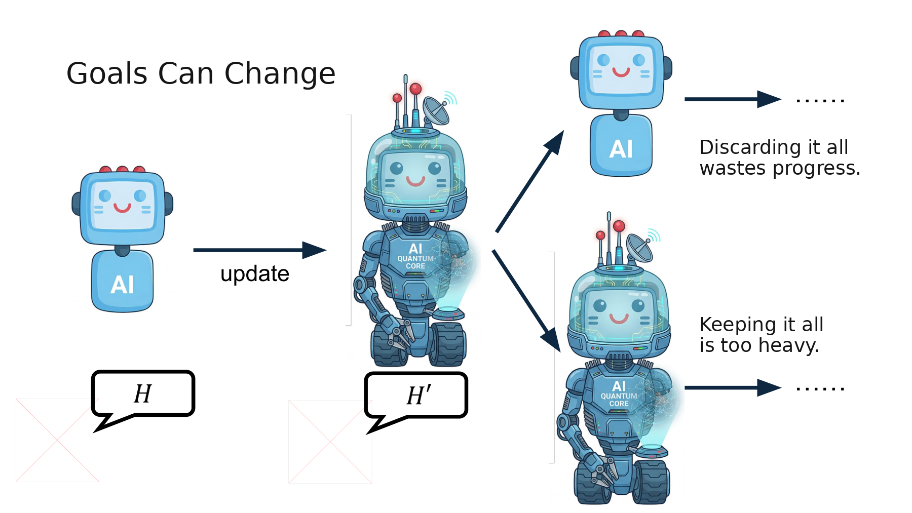
The robot on the left changes to meet goal H. In the middle, a new goal H′ splits its path. The robot above starts over with its original body. The robot below keeps the heavy equipment. Lee asks us to consider the radar. It can still serve the aircraft, even though the tracks would only weigh it down. Lee’s radar example, 27:29
The lecture moves from this analogy to speech recognition. It helps to ask what changed in each case. The robot’s criterion for success changes from traveling on the ground to flying. For speech recognition, success still means transcribing the words correctly. The background noise reaching the microphone changes the input distribution. We can therefore compare performance before and after adaptation using the same metric.
#Worked example · When does learning a new task raise the old task’s loss?
Translate the radar example into two weights. Keep a few examples of the earlier task A and call the gradient of their mean loss g_A. Call the gradient for the new task B g_B. A gradient points toward increasing loss, so an optimizer subtracts a chosen direction d scaled by the learning rate η. For a small step, a dot product approximates the change in A’s loss.
Take g_A = (1, 0), g_B = (−1, 2), and η = 0.1. Following B’s gradient increases the first weight by 0.1. That is precisely the weight whose increase raises A’s loss.
For A’s loss to stay level or fall to first order, the first coordinate of d must be at least zero. The closest vector to (−1, 2) satisfying that constraint is (0, 2). It removes the conflicting coordinate and keeps the second one.
A’s estimated change is zero, while B’s loss falls by about 0.4. This is a two-coordinate example of gradient projection in Gradient Episodic Memory (GEM). GEM checks a constraint for each earlier task using examples stored in memory. Those losses and full-task accuracy measure different things. Evaluate on held-out examples to see which skills survived. Lopez-Paz and Ranzato, NeurIPS 2017, Eqs. 7–8
#Part II, p. 27 — All three rows start with the same blue robot
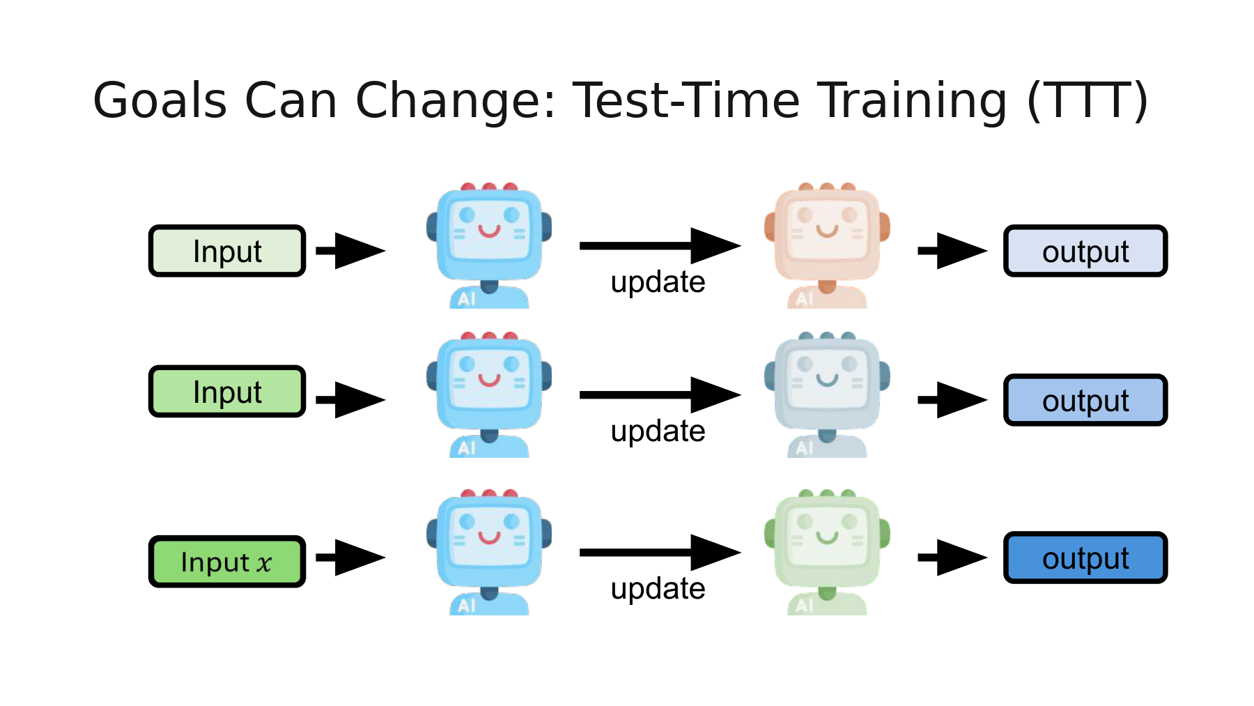
Read down the left side first. The inputs differ, but the model starts blue every time. Now read across any row: input → reference model → update → adapted model → output. The weights adjusted for the first input do not pass into the second row. Let θ₀ denote the reference weights, xₜ the current input, and A the adaptation procedure.
What can the model learn without the correct class label? In the vision experiments by Sun and colleagues, the program rotates an image by 0°, 90°, 180°, or 270°. It knows the angle it applied even when it does not know what object is in the photo. During training, object classification and rotation prediction share a feature extractor. At test time, the rotation loss updates the shared features. The object classifier then uses those features to read the original image. Imagine photographing a circular washer. If the image looks nearly identical under rotation, the angle provides little information. Which features the auxiliary task shares with the task we care about matters. Sun et al., ICML 2020, §2
#Worked example · Differentiate a rotation loss without knowing the object class
The program rotates the image by 90°. The model assigns one score to each of four angles. For a calculation we can do by hand, let z be the score (logit) of the known angle and hold the other three scores at zero. The 3 in the softmax denominator comes from three contributions of exp(0) = 1. Let p be the probability of the known rotation and let L be its negative natural log. Stanford CS231n, Softmax classifier
Initially z = 0. All four angles are equally likely, so p = 1/4 and L = ln 4 ≈ 1.3863. Differentiate the logarithm and the final term −z separately.
The slope is 0.25 − 1 = −0.75. With a learning rate of 0.4, subtracting that negative slope increases the score of the known angle.
The new loss is −ln p(z₁) ≈ 1.1701. This verifies a decrease in the loss for the known rotation. In TTT the chain rule carries this gradient back into the shared feature extractor. The calculation used no object label. Whether defect classification improved still requires a separate measurement. Sun et al., ICML 2020, Eqs. 2–3
#Supplementary lecture · What changes when a model spends longer on an answer?
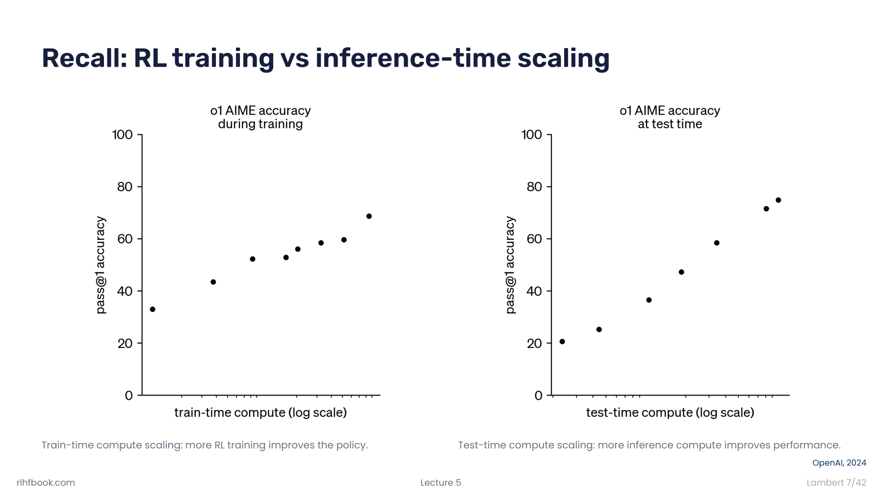
Nathan Lambert’s two plots have different horizontal axes. The left varies the compute spent training the policy. The right gives an already trained reasoning model more compute to answer a problem. In the recording, Lambert discusses the right-hand plot first, then returns to the left between 5:51 and 6:33. On the next slide, a sum-of-primes example shows the model using tokens to check candidate numbers and its arithmetic. The weights can stay the same for the next request. By comparison, implementing the update arrow on NTU’s page 27 requires a signal from the current input to change some parameters. Tracking generated tokens and weight updates separately tells us where computation went. Lambert, Lecture 5, slides 7–8 · Lecture video, 5:51
#Part II, p. 28 — Look at the model that starts the next row
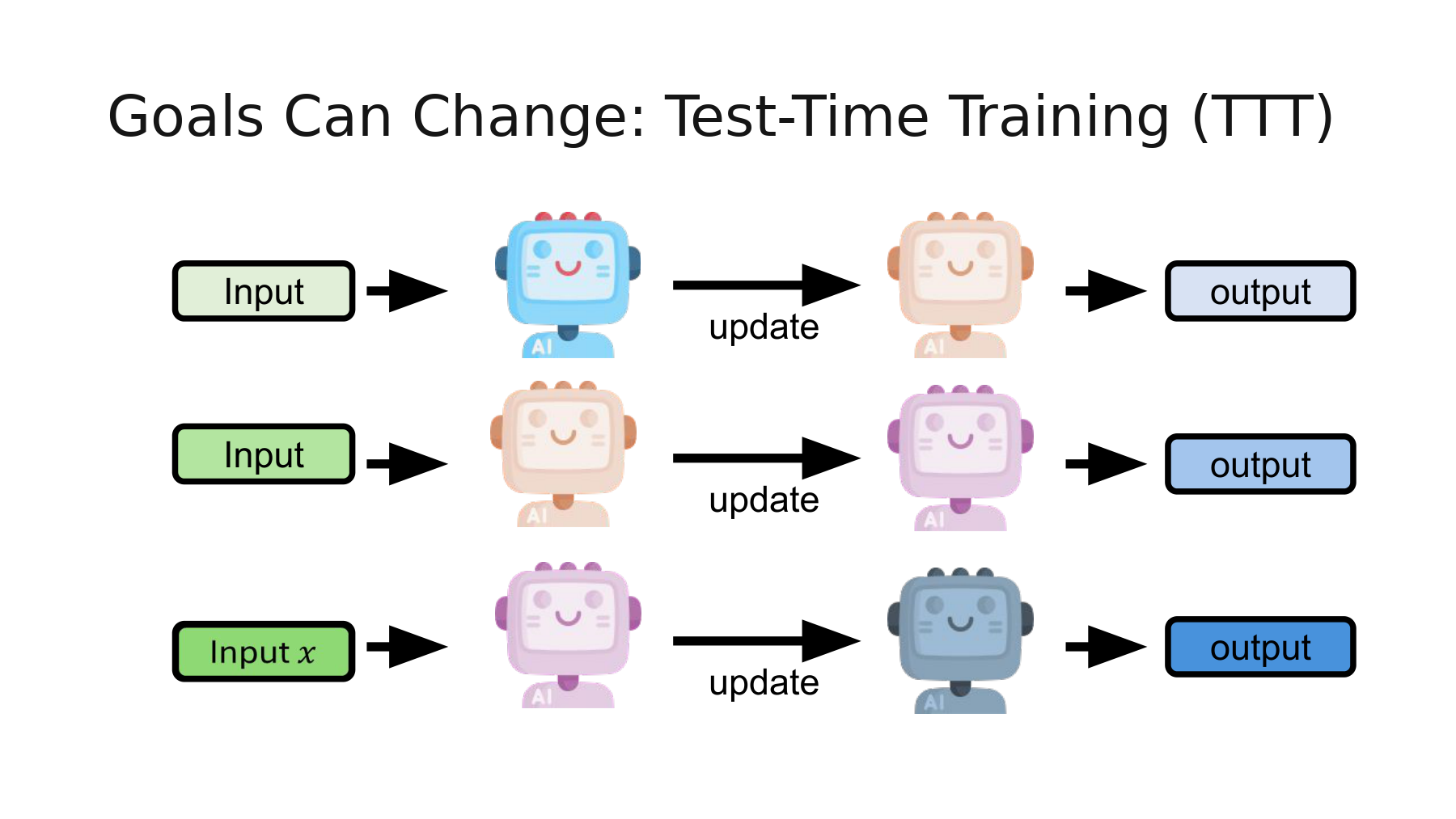
Compare the colors with page 27. The orange robot at the end of the first row reappears at the start of the second. The purple robot makes the same transition one row later. The adaptation procedure A is unchanged. Its first argument now holds the previous weights.
Let’s put numbers on the camera example. Imagine there is a brightness reference chart in view, and it gives us a target correction zₜ. The baseline correction is zero. On each frame, we move the current correction b halfway to the target. These are illustrative values.
| Frame | Target correction | Value after starting from zero | Value after starting from the previous correction |
|---|---|---|---|
| First frame from the dim camera | 4 | 2 | 2 |
| Second frame from the same camera | 4 | 2 | 3 |
| First frame from the bright camera | 0 | 0 | 1.5 |
On the second frame, the remaining errors are 2 and 1, respectively. Keeping the previous correction helped. On the third, the errors are 0 and 1.5, and the ranking reverses. Both procedures took one update per frame. The starting state explains the difference.
#Worked example · When does the correction error halve on each frame?
Replace the factor 1/2 in the table with a learning rate η. On the carry-forward path, bₜ = bₜ₋₁ + η(z − bₜ₋₁). Subtract the same target z from both sides and factor out the common term. As long as the lighting stays constant for t frames, we can substitute this relation t times.
Use target 4, initial value 0, and η = 0.5. The correction reaches 3 after two frames. On the third frame the target changes, so we stop using the closed form derived for target 4 and substitute the new target 0 into the one-step update.
With a fresh start on every frame, the first relation is applied only once each time. At the switch to the brighter camera, the reference value happens to equal the new target, giving zero error. If the darker scene continues instead, carry-forward halves its remaining error each time. That accounts for the change in ranking in the table.
#Supplementary paper · Which bars show the effect of carrying an image update forward?
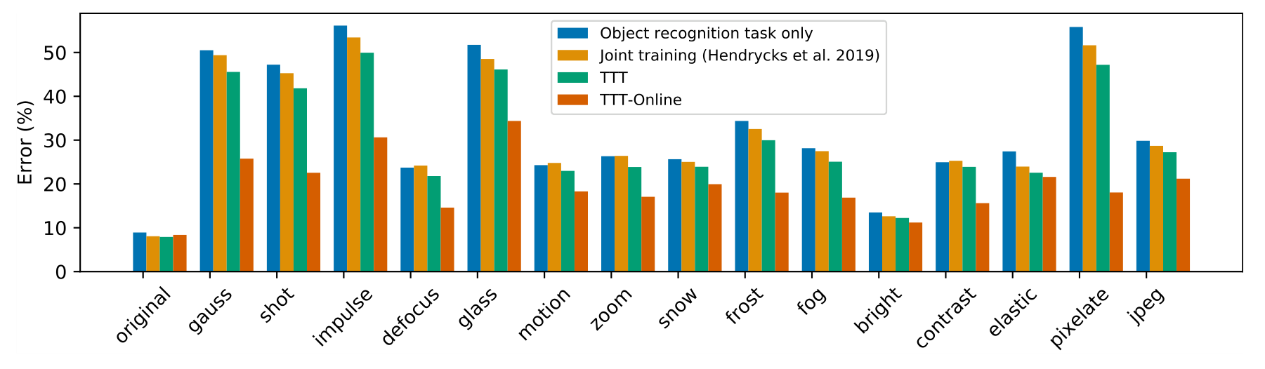
Choose one corruption on the horizontal axis and read the four bars in its group. The vertical axis shows classification error, so lower is better. The first two models were trained on object classification alone or jointly on classification and rotation prediction. The final two adjust features using test images. For the highest corruption severity, level 5, standard TTT resets and takes ten gradient steps per image. TTT-Online carries the updated state forward and takes one step per new image. The two bars differ in update budget as well as starting state. Comparing them tells us how the two procedures performed under the same type of corruption. To isolate the effect of retaining state, we would also need a comparison with matched step counts. To measure residual error immediately after switching cameras, we would need the order of corruptions and measurements taken just after the switch. Sun et al., Figure 1 and §3.1
#Part II, p. 29 — One model for this utterance, another to prepare for the next
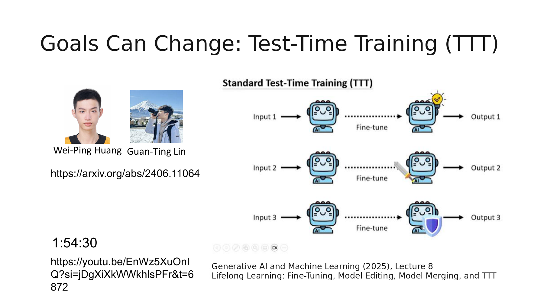
The diagram on the right starts each input from the same model. In the paper linked on the left, Lin, Huang, and Lee ask a follow-up question: How much of a quick adjustment made to hear one sentence should the next sentence inherit? In Lecture 8 from 2025, Lee distinguishes fast adaptation to one utterance from slower learning across several utterances. The time around 1 hour and 54 minutes printed on the slide belongs to that earlier recording. Lecture 8, 1:54:32 · Fast and slow updates, 1:56:16
#Supplementary paper · Two update speeds in DSUTA
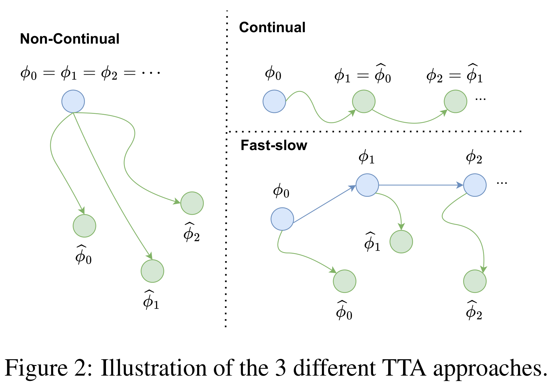
Dynamic SUTA (DSUTA) starts each utterance from a copy of the current reference weights. The fast update adjusts that copy several times on the current audio and uses it to produce a transcript. The slow update collects recent utterances in a buffer and updates the reference weights using their average adaptation loss. The next utterance starts from those reference weights. A final adjustment made for one unusual pronunciation can thus remain local to the utterance. The experiment uses reference transcripts to evaluate performance. Adaptation uses unlabeled speech and a loss computed from model predictions. Paper, §§3.1–3.2 and Algorithm 1
How does the model detect a change in noise? The dynamic reset procedure tracks how well the recent speech fits the model adapted to the earlier noise environment. Its indicator compares losses with those of the pretrained model. The procedure checks for a departure from the earlier range across multiple utterances before resetting the reference weights. It receives neither reference transcripts nor the true times at which the noise changes. Paper, §3.3
#Worked example · Detect a possible change without a reference transcript
In the DSUTA paper, L is a speech adaptation loss computed without labels. Evaluate the same utterance xᵢ with a reference model from the earlier environment, φ_D, and with the pretrained model, φ_pre. The paper calls the difference the Loss Improvement Index (LII). The order of subtraction matters. In the example below, −0.06 means the earlier environment’s model achieved a loss lower by 0.06.
Suppose the four latest utterances give indices −0.06, −0.02, 0.00, and +0.04. The mean is still negative. To tell whether conditions have deteriorated, compare it with the mean recorded in the previous environment.
Let the previous mean μ be −0.10 and its standard deviation σ be 0.08. For M = 4 utterances, the calculation uses a standard error of 0.08/√4. Substituting into the paper’s buffer-average rule gives the following value.
The statistic 2.25 exceeds the paper’s threshold of 2. The adapted reference still has a small average advantage over the pretrained model, but much of the advantage it used to have has disappeared. This establishes one threshold crossing. The implementation also uses a patience condition to handle transient changes. Strong correlations between successive utterances can make the standard error of their mean larger than expected. The statistic itself gives no probability that the noise changed. Lin et al., §3.3 and Appendix Algorithm 2
Word error rate (WER) counts the substitutions S, deletions D, and insertions I needed to match a reference transcript, then divides by the number of reference words N. Two substitutions, one deletion, and one insertion against a 20-word reference give a WER of 20%.
The denominator counts the 20 reference words. A word added by the model increases only the numerator.
| Method in Table 2 | State retained for the next utterance | MD-Hard WER ↓ |
|---|---|---|
| Source model | Fixed pretrained weights | 74.6% |
| SUTA | Return to pretrained weights for each utterance | 60.4% |
| CSUTA | Weights adapted on the preceding utterance | 83.6% |
| DSUTA | Reference weights updated on batches of recent utterances | 45.6% |
| DSUTA + Fixed reset | Reset reference weights at fixed intervals | 49.4% |
| DSUTA + Dynamic reset | Reset when the loss indicator signals an environment change | 39.8% |
These are means over three runs on MD-Hard, a stream with changing noise conditions. Adding dynamic reset to DSUTA reduced WER from 45.6% to 39.8%, a 5.8 percentage-point drop. Resetting the same method every 50 utterances raised WER by 3.8 points to 49.4%. Carrying every update forward (CSUTA) put WER 9.0 points above the fixed model. These results describe transcription on the changing stream. Measuring retention in a previous environment requires evaluating the model again on a separate set from that environment. Lin et al., EMNLP 2024, Table 2
The change from 45.6% to 39.8% can also be reported as a relative error reduction. The denominator is the WER of DSUTA before adding dynamic reset, 45.6%.
Using the rounded entries in the table, the absolute difference is 5.8 percentage points and the relative reduction is about 12.7%. The two calculations use different denominators.
#Part II, p. 30 — After teaching a new skill, ask for the old one again
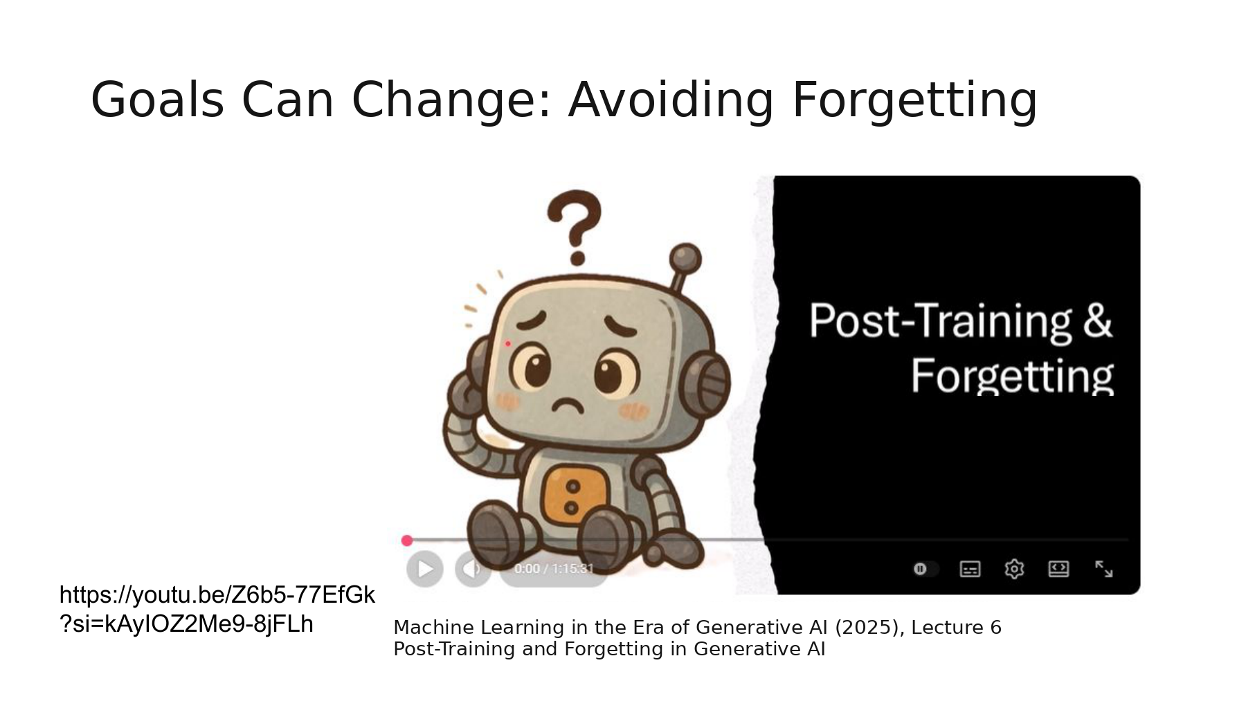
Lee recalls that repeated weight updates can erode a previously learned skill. He then asks what happens if only the harness changes, for example through a new system instruction or a change to external memory. The diagnostic differs. Suppose an agent stops reporting units after an instruction edit. Give it the same input and weights, and restore the previous instruction. If the units return, the instruction change explains the behavioral difference in this case. NTU lecture, 30:18
#Supplementary lecture · Rehearse on old examples and evaluate on held-out ones
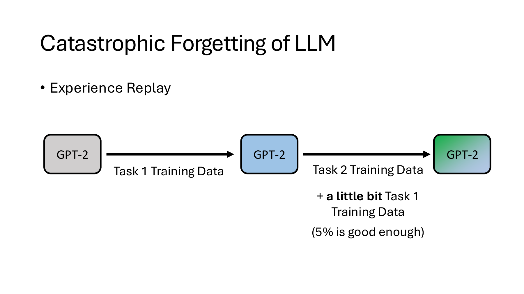
Pages 28–30 of the 2025 post-training lecture compare sequential fine-tuning, a regularization method that limits changes to important weights (MAS), and experience replay. Follow the plus sign on the middle slide: add a sample of old training examples to the training set for the new task. Revisiting those original inputs and targets can help preserve a mapping the model might otherwise lose. Lee’s example adds about five old examples per hundred new training examples. A suitable replay ratio depends on how much data can be retained and how closely the tasks resemble each other. Lecture 6, 42:56 · Slides 28–30
How would we check for forgetting in a vision system? Set aside separate training and evaluation images for each of two cameras, A and B. The hypothetical results below compare predictions on the same held-out images before and after adaptation on camera B’s training data. Only A’s training images can go into the replay buffer. Its evaluation images remain held out throughout.
| Same held-out evaluation set | Before adapting to B | After adapting to B | Accuracy change |
|---|---|---|---|
| Original camera A | 90% | 82% | −8 percentage points |
| New camera B | 60% | 78% | +18 percentage points |
The new camera gained 18 points and the original camera lost 8. To measure the effect of replay, start two runs from the same model. Use only B’s training images in the first. Mix in some of A’s training images in the second. Give both runs the same update budget, then measure both models on the same held-out A and B sets. This gives separate readings for retention and adaptation.
#Worked example · How much forgetting does a final accuracy of 80.3% conceal?
Read the table above as a history of learning two tasks. The GEM paper’s backward transfer (BWT) metric compares accuracy just after a task was learned with accuracy on the same evaluation set after the final task. With just one earlier task A, BWT is 82 − 90 = −8 percentage points. The +18 points on B measure adaptation to the new task. GEM, Eqs. 2–4
Now introduce a third camera C. Each row marks the point just after learning from that camera. Each column uses a fixed test set from one camera. The diagonal gives each camera’s accuracy immediately after learning it. The row for C is hypothetical.
| Training completed through | Accuracy on A | Accuracy on B | Accuracy on C |
|---|---|---|---|
| A | 90% | — | — |
| B | 82% | 78% | — |
| C | 86% | 71% | 84% |
Read the last row across for the final performance. If each camera gets equal weight, average accuracy (ACC) is as follows.
To measure forgetting, read down each column. A fell from 90% when learned to 86% at the end. B fell from 78% to 71%. Average these two changes. C has experienced no subsequent task, so it does not enter the denominator.
On A, accuracy recovered by 4 percentage points since the preceding checkpoint. It still sits 4 points below its value just after learning A. Recovery and residual forgetting can coexist because their reference times differ. The final average of 80.3% does not expose that history.
The blue starting models on page 27, the colors passed between rows on page 28, and the slowly updated reference model on page 29 each answer the same question: Which changes made for this input should the next input inherit? Episode 20 continues on page 31 of the second lecture.