For AI to study on its own, it must generate problems to solve and obtain a trustworthy learning signal from its attempts.
Part 13, the conclusion of the first half, distinguished model weights, the harness, and memory accumulated during execution. The second half asks what evidence would justify saying that this agent has improved. If AI writes the questions, supplies the answers, and evaluates them, where can we check for genuine improvement?
Start with three roles. The proposer creates the next learning problem, the solver attempts it, and the verifier turns the answer into a learning signal. To understand the loop, first distinguish the human objective, the loss used to update the model, and the evaluation used to measure improvement.
This article follows slides 1–5 of the second lecture. Lecture slides and videos from Nathan Lambert and CMU provide context on proxy objectives, synthetic data, and learnable difficulty. Figures from Absolute Zero, R-Zero, SPICE, and R-Few illustrate different sources of learning signals.
Worked examples Problem mix · Reward and probability · Attempts and difficulty
Video locations by slide
The links mark where discussion of each topic begins.
| Slide | Video | Topic |
|---|---|---|
| Second half, 1 | From 0:00 | The question behind the second lecture |
| Second half, 2 | From 0:07 | Recursive improvement in which AI builds better AI |
| Second half, 3 | From 0:45 | Objectives, human-provided information, and training loss |
| Second half, 4 | From 3:36 | Parameter updates and hoped-for evaluation gains |
| Second half, 5 | From 4:45 | The proposer–solver–verifier loop |
#Second half, slide 1 — What does it take to learn independently?
Independent study involves more than repeatedly generating answers. A learner selects problems that address weaknesses, attempts them, judges which attempts helped, and uses that judgment to shape subsequent training. Humans, the model itself, and the external environment can all supply information for this process.
When a study reports less human intervention, ask which activities it automated. Writing new problems, assigning correct answers, adjusting difficulty, updating a model, and conducting the final evaluation are distinct tasks. Automating one does not settle the others.
Suppose a model writes its own remainder problem. It asks for the remainder of 17 divided by 5, answers 3, and gives itself a pass. The log contains a question and a reward but no clue to the error. An arithmetic check gives 17 = 5 × 3 + 2: the 3 is the quotient and the 2 is the remainder. When reading the question on the title slide, ask what information could overturn the model’s first answer. Here it comes from the division rule.
#Second half, slide 2 — Recursive improvement is a research hypothesis
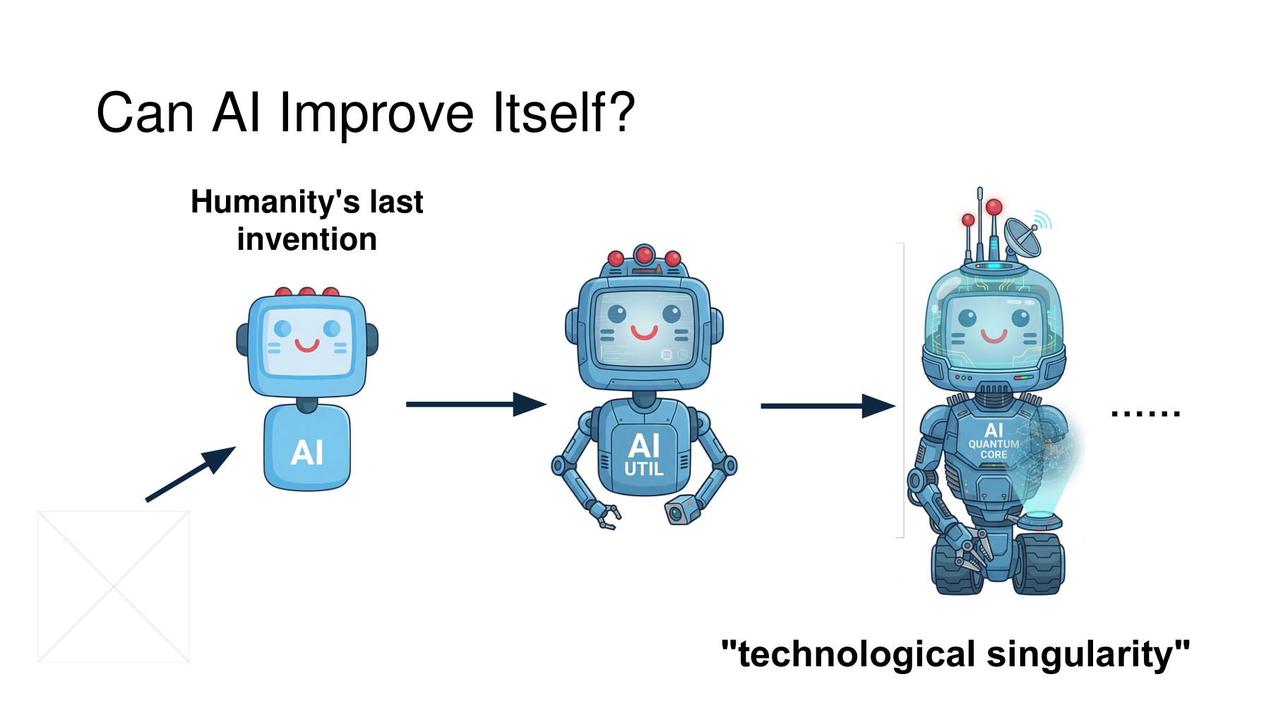
The slide depicts a human-built AI producing a better AI, which then improves the next one. The lecturer connects this possibility to the technological singularity. The diagram is a proposal about what might happen if improvement could continue. It is not experimental evidence for unlimited gains. Lecture at 0:07
Experiments require more specific questions. Does a trained model perform better under the same conditions? Can it generate better problems for the next training round? Does repetition correct errors or reinforce them? To give recursive improvement a testable meaning, identify what actually changes at each arrow.
Imagine keeping a human-written problem generator frozen while updating only the solver three times. Scores of 60, 70, and 74 on the same test can rise with the generator’s capabilities unchanged. To probe the next arrow in the diagram, ask whether a better model can train the next generation more effectively. Use the earlier and later model as proposers. Start two identical copies of a fresh solver, give each proposer the same problem-generation budget, and train both solvers for the same number of updates. Their scores on a fixed test hidden from the proposers can then tell us something about the ability to teach the next solver.
#Second half, slide 3 — Separate the objective, training information, and evaluation
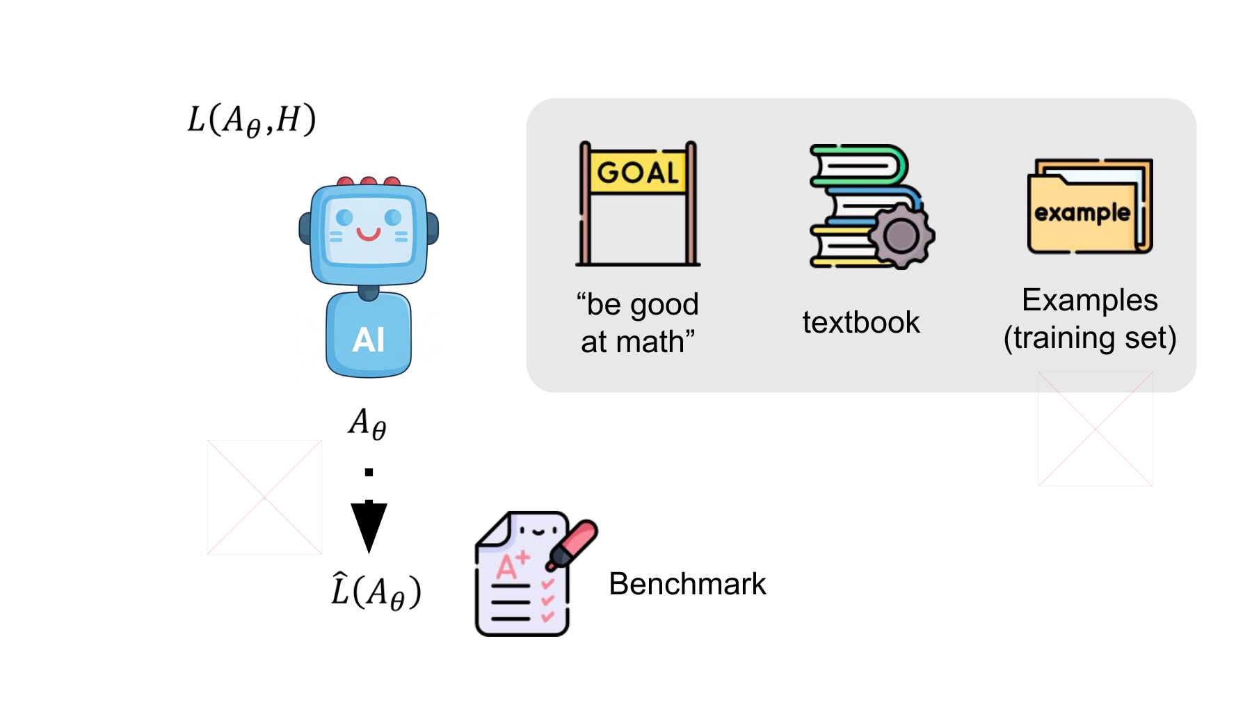
The lecturer writes Aθ for an AI with parameters θ and L̂ for an evaluation of the desired outcome. In research, a benchmark often stands in for this evaluation. Counting errors on specified problems is more concrete than asking a model to “get better at mathematics.” A single benchmark still captures only part of mathematical ability. Lecture, 0:45–2:01
The training loss L also uses information people provide. The goal instructions, textbooks, and examples on the right of the slide are instances of this information. The lecturer calls it H. To distinguish it from the harness H in Part 13, this article uses H_info for human-provided information. Lecture at 2:30
| Symbol | Meaning here | Question to ask |
|---|---|---|
| θ, Aθ | The model parameters and the AI using that model | What did training change? |
| H_info | Human-provided information such as instructions, documents, and examples | How does the information describe the desired capability? |
| L | The loss that guides training | What quantity does the model update seek to reduce? |
| L̂ | Evaluation loss that measures progress toward the objective | Did the capability improve under new conditions? |
H_info is a proxy for the intended objective. Give a model a few arithmetic examples and it may learn their wording instead of the underlying procedure. Even with a textbook, the skills learned depend on which passages become problems. This makes the relationship between human input, the learning signal derived from it, and the final evaluation important.
Here, smaller values of both L and L̂ are better. Other metrics, such as accuracy, reward larger values. Retain the loss convention when reading the lecture’s inequality.
#Did the solver improve, or did the proposer supply more easy questions?
Suppose the proposer writes both the training questions and the progress checks. The first check contains 50 easy and 50 hard questions. The solver gets 45 and 20 right, respectively. On the next check it gets 68 out of 80 easy questions and 7 out of 20 hard ones. The total rises from 65 to 75. Which part of the second arrow on slide 2 improved?
Let w be the fraction of easy questions and let the two a values be accuracy within each group. Multiplying each accuracy by its group’s share gives the overall score. Higher accuracy is better here.
Accuracy fell from 90% to 85% on easy questions and from 40% to 35% on hard ones. Reusing the first check’s weights gives the second solver 60%. Its self-generated score rose 10 percentage points while its score at fixed weights fell 5 points. WILDS evaluates performance in familiar and new environments, including shifts across hospitals and camera locations. Here we apply that evaluation principle to question types. Reweighting still assumes comparability within each type. Testing both solvers on the same independently held-out questions would control for a change in difficulty within a type as well. Koh et al., WILDS, ICML 2021
#Second half, slide 4 — Reducing training loss and improving ability
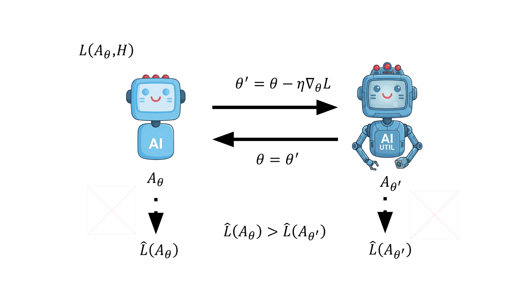
Once a training loss is defined, model parameters can be updated. The slide illustrates one gradient descent step. η is a positive learning rate, and ∇θL is the gradient, indicating how the loss changes with a small change in the parameters.
The update aims to reduce L. A large learning rate or a complex loss surface can prevent L from falling on a given step. Even when L falls, the desired evaluation outcome must be checked separately. When introducing the inequality below, the lecturer says we hope the model performs better after the update. Lecture at 3:55
Gradient descent does not imply this inequality. It depends on how well the data represent the objective, how accurately the reward measures answer quality, and whether repeated training adapts to only a narrow set of problems.
#Worked example 1 — Training loss can fall while evaluation loss rises
Consider a hypothetical one-parameter model. The values are illustrative. Training favors θ=1, while evaluation favors θ=−1.
Initially θ=0. With a learning rate of 0.25, the training loss gradient is −2, giving this update:
Substitution of the values before and after the update shows the losses moving in opposite directions.
Training loss falls by 0.75 and evaluation loss rises by 1.25. This is a counterexample showing that even accurate optimization of a proxy can fail if it points away from the intended objective. When a system generates its own problems and verifies answers automatically, designing the link between these objectives becomes part of its architecture.
Also consider how evaluation data are used. If the same benchmark influences the problem generator or model selected each round, it supplies information during development. Testing final generalization requires data and conditions that played no role in selection. Keeping answers out of the model’s direct view is insufficient to make an evaluation independent.
#A related lecture — How do overfitting and overoptimization differ?
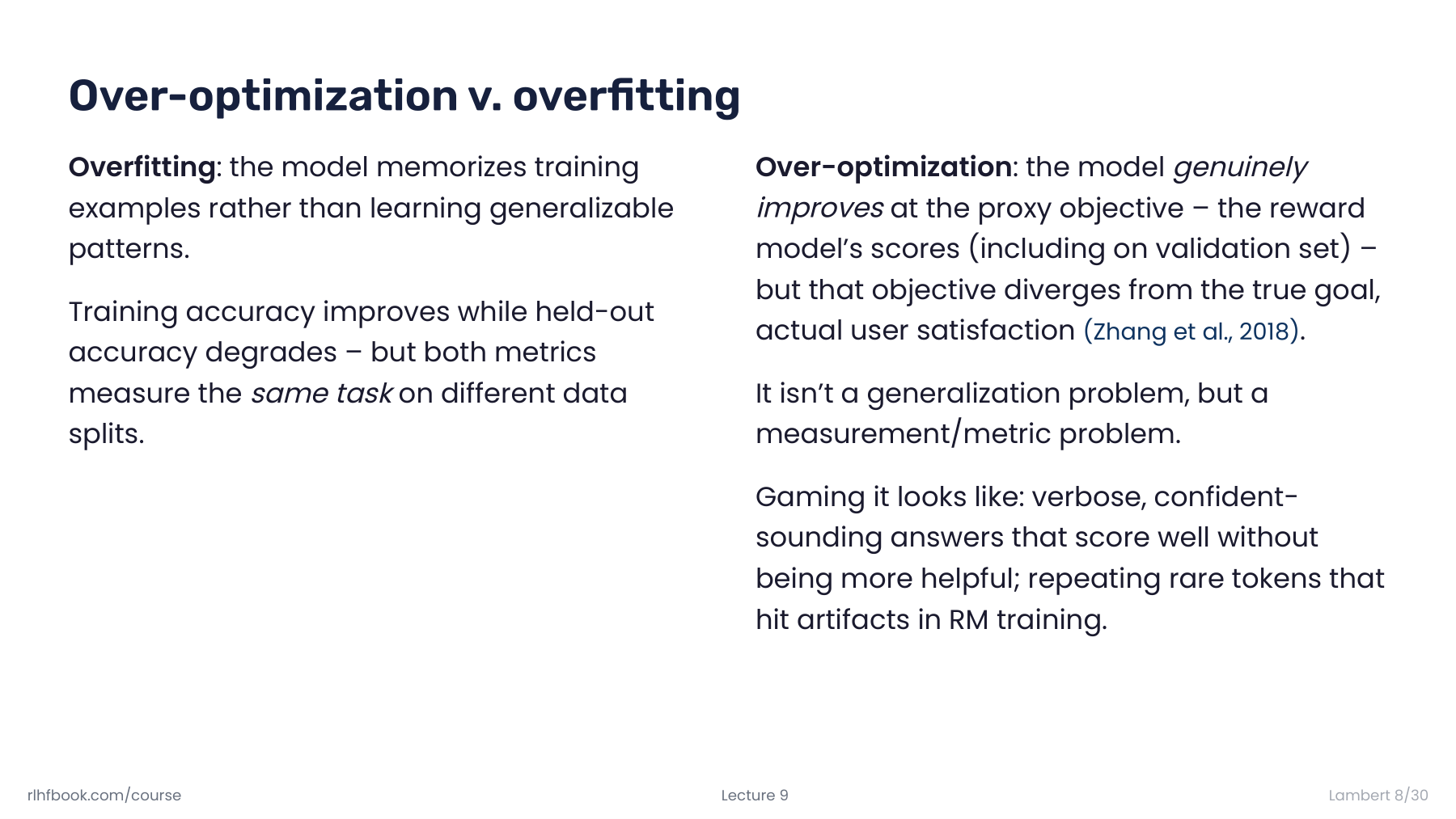
Lambert distinguishes overfitting from overoptimization. In a typical case of overfitting, gains on training data fail to carry over to new examples of the same task. In overoptimization, the model may genuinely get better at maximizing a proxy while its results move farther from the intended goal. Slide 8 · Video, 05:39–06:35
| Problem | Quantities compared | Question to ask |
|---|---|---|
| Overfitting | Training and held-out examples of the same task | Does the learned pattern apply to new data? |
| Overoptimization | Optimized proxy metric and true objective | Does a higher score indicate a stronger target capability? |
Apply this distinction to self-learning. Suppose a verifier rewards answer length more strongly than accuracy. If the solver writes lengthy answers on new tasks too, verifier scores may rise on both training and validation tasks. Those scores alone cannot tell us whether errors decreased. This hypothetical example illustrates metric misalignment.
Revisit the quadratic example. It contains no assumption that the model memorized training sentences. Its losses diverge because training and evaluation favor different directions. Testing the inequality on slide 4 therefore requires both partitioning the data and scrutinizing the evaluation criterion. Check answer accuracy or task success independently of the verifier used in self-learning to determine whether the model merely adapted to that verifier’s preferences.
In practice, overfitting and metric misalignment can coexist. Distinguishing them helps choose a diagnostic for the cause. If a verifier consistently favors length or tone across data splits, examine the criterion itself.
#Second half, slide 5 — The proposer, solver, and verifier form a learning loop
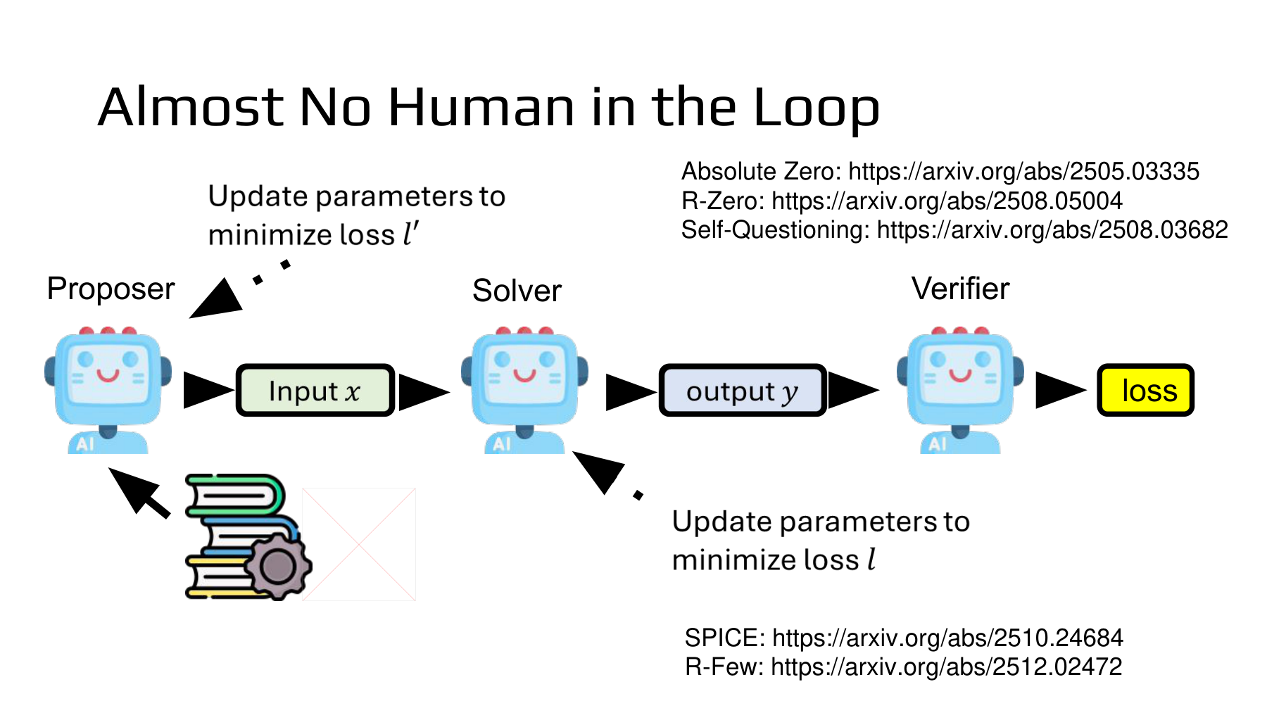
From 4:45, the lecturer introduces a structure that reduces the need for ongoing human intervention. The proposer creates problem x, the solver produces answer y, and the verifier returns a learning signal. The slide shows separate losses for the two policies because generating a useful problem and solving a given problem are different objectives.
Write q for a problem, φ for the proposer’s parameters, and θ for the solver’s parameters. z is context for problem generation, such as a document or previous problem, and V maps the answer to reward r. This notation describes a shared structure rather than any one paper’s full algorithm.
The solver can learn to increase the expected reward of its answers. During the update below, take the proposer that generates q and the verification rule as given.
Language models output discrete tokens. This does not mean differentiating the verifier score directly with respect to a token. Reinforcement learning uses the reward for a generated output to adjust how likely that output is. The proposer needs its own signal, for instance whether the solver can learn at this difficulty and whether the problems are sufficiently diverse.
The three roles do not require three distinct language models. One model can alternate between proposing and solving. The verifier might be a code executor or a rule that compares answers. Alternatively, the proposer and solver can have separate weights. The four studies below illustrate these choices.
#How far can a reward move the probability of an answer?
Slides 19–20 of the CMU lecture differentiate a reward averaged over the probabilities of entire trajectories. To work through the idea, reduce all solutions to one question to two choices, A and B. The verifier gives the correct answer A a reward of 1 and the incorrect B a reward of 0. Let p be the probability of A and z its log odds, so p is the sigmoid σ(z). At p = 0.25 the opening odds are one to three. CMU Lecture 9, policy gradient derivation, pp. 19–20
The update uses a learning rate of 0.8 and steps toward higher expected reward. A’s probability rises from 25% to about 27.9%. There is no need to differentiate the answer itself. The reward difference and the probabilities assigned to the two choices determine the update. We could compute the exact expectation because this illustrative policy has two known choices. Language models estimate the gradient from sampled trajectories. If the verifier gives both answers equal rewards, the first factor in the derivative is zero and this question supplies no preference between them.
#A related lecture — Synthetic data can supply questions, answers, and judgments
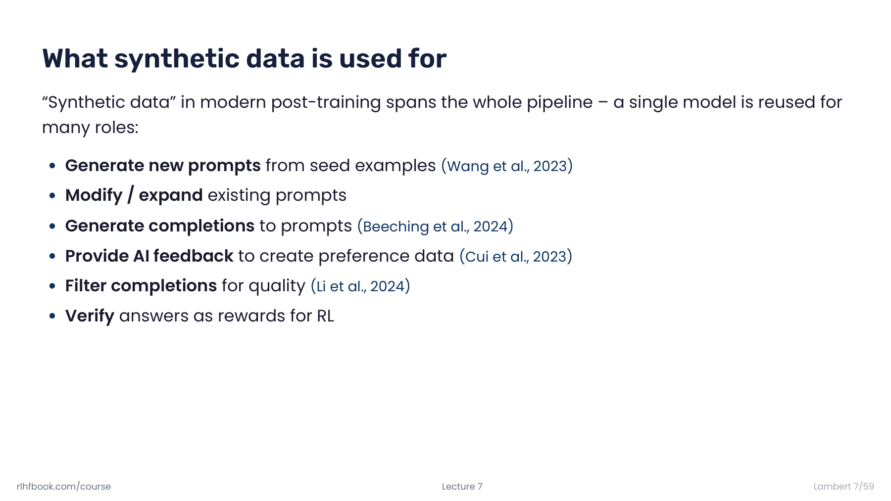
Lambert’s lecture on synthetic data explains how model-generated material enters different stages of training. A model can use seed examples to generate new questions, answer those questions, and generate judgments of answer quality or preference. A single model can serve several of these functions. Slide 7 · Video, 03:29–05:35
The following table maps these ideas onto the three roles in the NTU lecture.
| Material generated in Lambert’s lecture | Corresponding NTU role | Quality check |
|---|---|---|
| New and revised questions | The proposer supplies learning problems | Are the questions clear and relevant to the target skill? |
| Responses to questions | The solver generates candidate answers for training | Are they correct? Do they include different solutions? |
| Preference, quality, and verification signals | The verifier informs answer selection and rewards | Are higher scores associated with correct answers? |
Suppose a model writes a question based on a document, answers it, and grades its own answer. Saying that AI generated the data leaves the process underspecified. Inspect the question’s basis, the answer, and the grading criterion separately. If all three stages share a misconception, a plausible problem, a plausible answer, and a high score can all arise together. Assigning three roles and obtaining verification evidence with independent errors are distinct design challenges.
After generation, decide what to retain and how to use it in parameter updates. Lambert discusses filtering recurrent outputs. Video, 07:22–07:35 Selection changes the training distribution of questions and answers. Keeping only similar answers can reduce diversity, while a flawed acceptance criterion can increase training on incorrect answers.
For all four studies, ask where problems come from, how answers are verified, and which data are used for the next update. The external documents in SPICE and the anchor examples in R-Few add reference information at different points.
#Supplement A — Absolute Zero uses an executable environment to ground answers
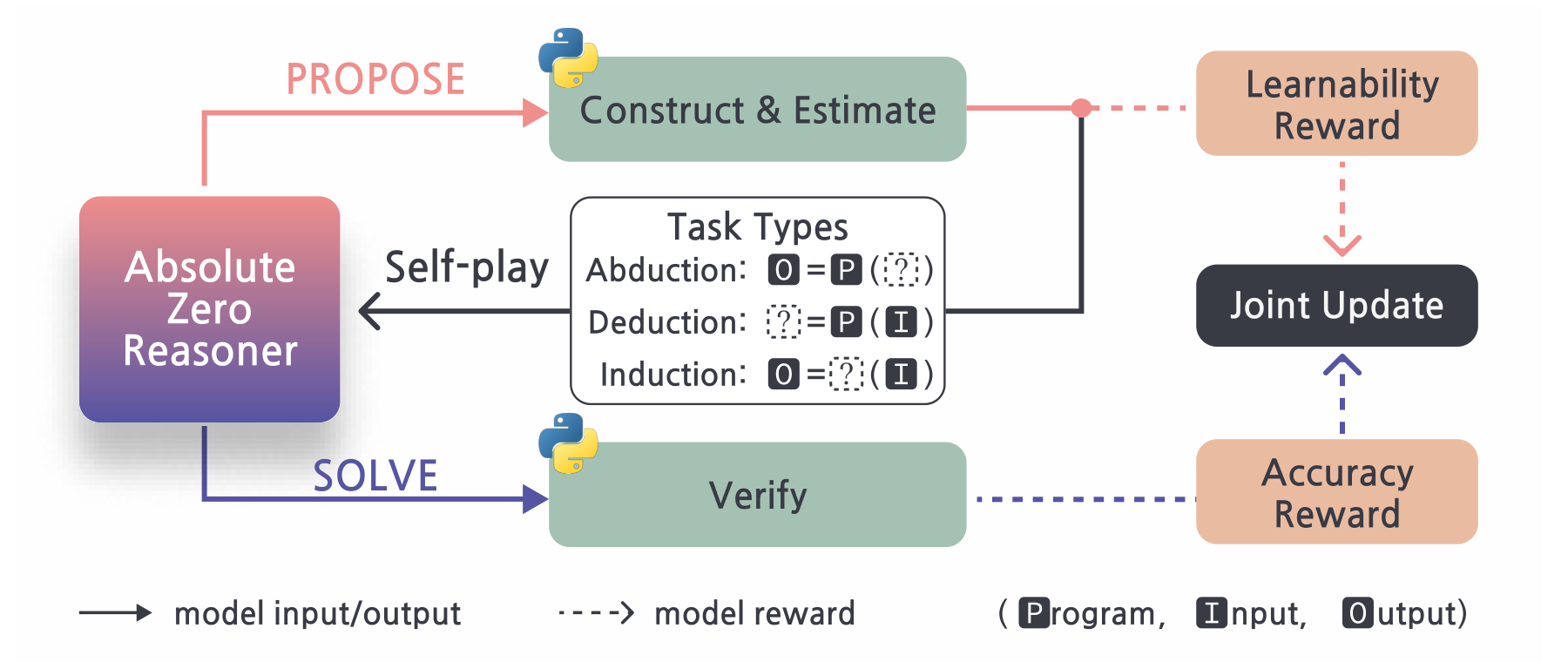
Absolute Zero Reasoner (AZR) uses a single model as proposer and solver. Tasks describe relationships among programs, inputs, and outputs. A code executor checks the validity of proposed tasks and verifies answers. Training covers deduction (predict the output), abduction (find an input that produces an output), and induction (construct a program from input–output examples). Absolute Zero, section 3 and Figure 4
For example, if a program doubles an input and adds 3, execution can verify that input 4 produces 11. In program induction from a few examples, however, several programs can pass the same examples. An executor verifies what it tests. It does not prove that an answer meets every intended requirement. The inputs and conditions examined define the scope of verification.
The solver’s base reward checks whether its answer has the same value as the verified answer. The indicator below returns 1 if the condition holds and 0 otherwise. The environment provides the reference answer y*, and this reward tests equality of Python values. Absolute Zero, section 3.1, equation 5
A proposer that simply causes frequent failures is of limited use. A problem that the solver never solves provides no successful trajectory to learn from. AZR uses the mean success rate p̄ over multiple attempts to define the following base reward.
Suppose a valid task is attempted 10 times. For 0, 1, 5, 9, or 10 successes, the proposer receives base rewards of 0, 0.9, 0.5, 0.1, or 0, respectively. Difficult tasks with at least one observed success score highly. This expression does not peak at a 50% success rate. Ten failed attempts also do not prove a task is impossible. Absolute Zero, equation 4
These are the base rewards for the two roles. The paper adds penalties for formatting and incorrect answers. “Zero Data” means this training stage does not rely on externally annotated tasks with answers. It still uses a pretrained model, designed task types, a code execution environment, and a seed triple for the identity function at initialization. Absolute Zero, equation 6 and section 3.3.1
#Would four attempts and ten attempts favor the same problem?
In Equation 4 of Absolute Zero, a proposer receives zero if the solver records no successes. Its expected reward therefore depends on how often a task is attempted. Assume each of K independent attempts on one problem succeeds with a fixed probability p. The number of successes X is binomial. If every outcome first receives 1−X/K, the mean is 1−p. That temporary rule awards 1 when X is zero. Subtract the probability of that event to recover the paper’s rule. Absolute Zero, Equation 4
| Attempts on one problem | Hard problem, p=0.1 | Moderate problem, p=0.5 |
|---|---|---|
| 4 | 0.9−0.9⁴ = 0.2439 | 0.5−0.5⁴ = 0.4375 |
| 10 | 0.9−0.9¹⁰ ≈ 0.5513 | 0.5−0.5¹⁰ ≈ 0.4990 |
In four attempts, the hard problem produces no success 65.61% of the time. With ten attempts that probability drops to about 34.87%, reversing the expected reward ranking. The proposer’s learning signal changes even with the same solver ability. These are illustrative values derived from the paper’s base reward. Duplicating an answer or showing the next attempt an earlier solution breaks the independence assumption behind the table.
#A related lecture — What can a solver learn from tasks that are too easy or too hard?
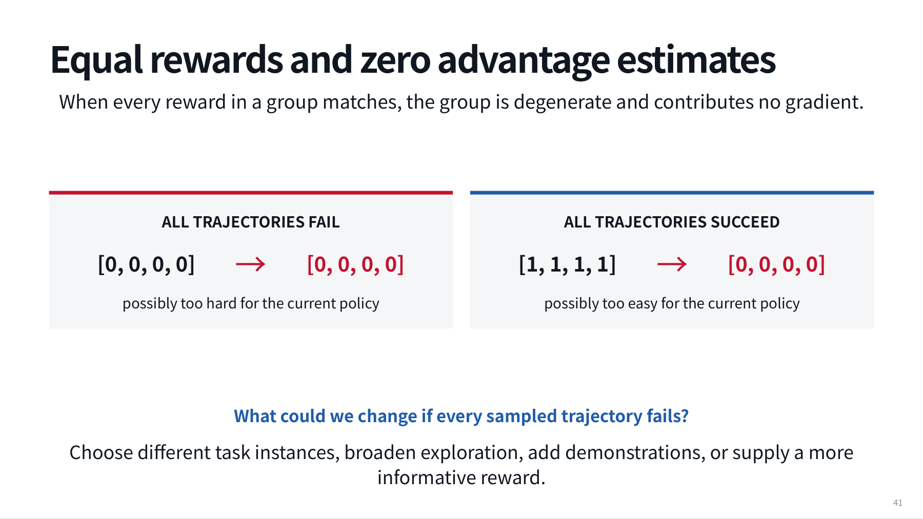
CMU’s introductory reinforcement learning lecture offers another reason to select problems the current solver can learn from. Sample several answers to the same question and subtract the group’s mean reward from each individual reward. This compares each answer with its peers and can help estimate relative advantage. Slides 37–41
The table shows only the reward minus its group mean. A full GRPO objective can also involve normalization, policy probability ratios, and clipping.
| Rewards for the same problem | Group mean | Each reward minus the mean |
|---|---|---|
| 0, 0, 0, 0 | 0 | 0, 0, 0, 0 |
| 1, 1, 1, 1 | 1 | 0, 0, 0, 0 |
| 1, 1, 0, 0 | 0.5 | 0.5, 0.5, −0.5, −0.5 |
If every attempt fails, the problem may be too difficult. If every attempt succeeds, it may already be familiar. In both cases there is no within-group reward difference, so the relative policy update term based on these outcome rewards cannot distinguish solutions. A KL regularizer or auxiliary loss can still produce gradients. Implementations that normalize by standard deviation must also handle a group with zero variance. Slide 41 · Video, 1:13:46–1:14:29
Compare this with the AZR proposer reward. CMU describes the signal for updating the solver. AZR’s rule determines which problems the proposer is encouraged to create. Generating more tasks with no observed chance of success may still produce no successful examples to learn from. A proposer should supply problems worth attempting at the solver’s current level.
There is no universal conclusion that 50% accuracy is optimal. AZR’s own base proposer reward does not peak there. When all attempts fail, the CMU lecture suggests selecting another task, adding guidance or demonstrations, changing the starting point, or using a more informative reward. Video, 1:14:33–1:15:07 Difficulty, exploration, initialization, and verification signal are all adjustable.
#Supplement B — R-Zero feeds solver uncertainty back into problem generation
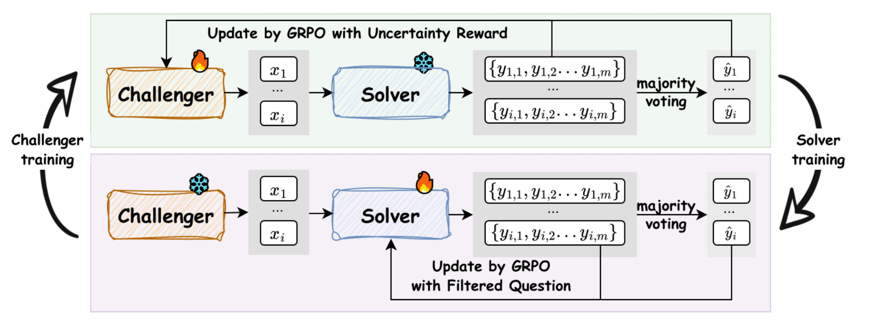
R-Zero initializes a challenger and solver from the same base model and optimizes them separately. First it freezes the solver and trains the challenger to create suitable questions. It then filters the challenger’s questions and uses them to train the solver. R-Zero, sections 2.1–2.4
The solver samples several answers to a problem. Their most frequent value becomes a pseudo-label in place of a reference answer from a code executor. Let ỹ denote this label and m the number of answers generated for one question. Then p̂ is:
Here p̂ measures agreement with the solver’s own most frequent answer. It does not measure accuracy against an external answer. The paper uses p̂ to compute an uncertainty reward. Moderate agreement earns a high reward, discouraging a challenger from generating only questions on which the solver is already confident. R-Zero, section 2.2
#Worked example 2 — A difficulty reward does not certify an answer
Compare hypothetical sets of 10 responses per problem. Assume every problem passes the format checks. For a question in cluster C of similar questions within a batch of size B, R-Zero also applies a repetition penalty proportional to the cluster’s share of the batch.
Set B=20, the cluster size to 4, and λ=1, making the repetition penalty 0.2 in every row. The batch and cluster sizes are illustrative. R-Zero repetition penalty · Combined reward
| Hypothetical problem | Frequency of the most common answer | p̂ | Uncertainty reward u | Reward after repetition penalty |
|---|---|---|---|---|
| A | 3 / 10 | 0.3 | 0.6 | 0.4 |
| B | 5 / 10 | 0.5 | 1.0 | 0.8 |
| C | 7 / 10 | 0.7 | 0.6 | 0.4 |
| D | 10 / 10 | 1.0 | 0.0 | 0.0 |
With more than two distinct responses, the most frequent answer can have just a 30% share, as in A. If five responses occur 3, 2, 2, 2, and 1 times, the first is the mode. What the paper calls majority voting need not produce an absolute majority.
Suppose problem C asks for 17×23. If 381 appears seven times, the correct answer 391 twice, and 401 once, then p̂=0.7 while actual accuracy is 0.2. Rewarding agreement with the pseudo-label 381 can reinforce an incorrect consensus. The reward of 0.4 measures the example’s difficulty and repetition criteria. It provides no evidence that 381 is correct.
R-Zero filters generated questions by agreement before training the solver. Filtering aims to improve task quality, but external verification of correctness is a separate matter. The paper also reports intervals in which performance deteriorated after further rounds of self-evolution. Sustaining improvement takes more than running the loop longer. R-Zero, section 2.3 · Section 4.2
#Supplement C — SPICE grounds questions and reference answers in external documents
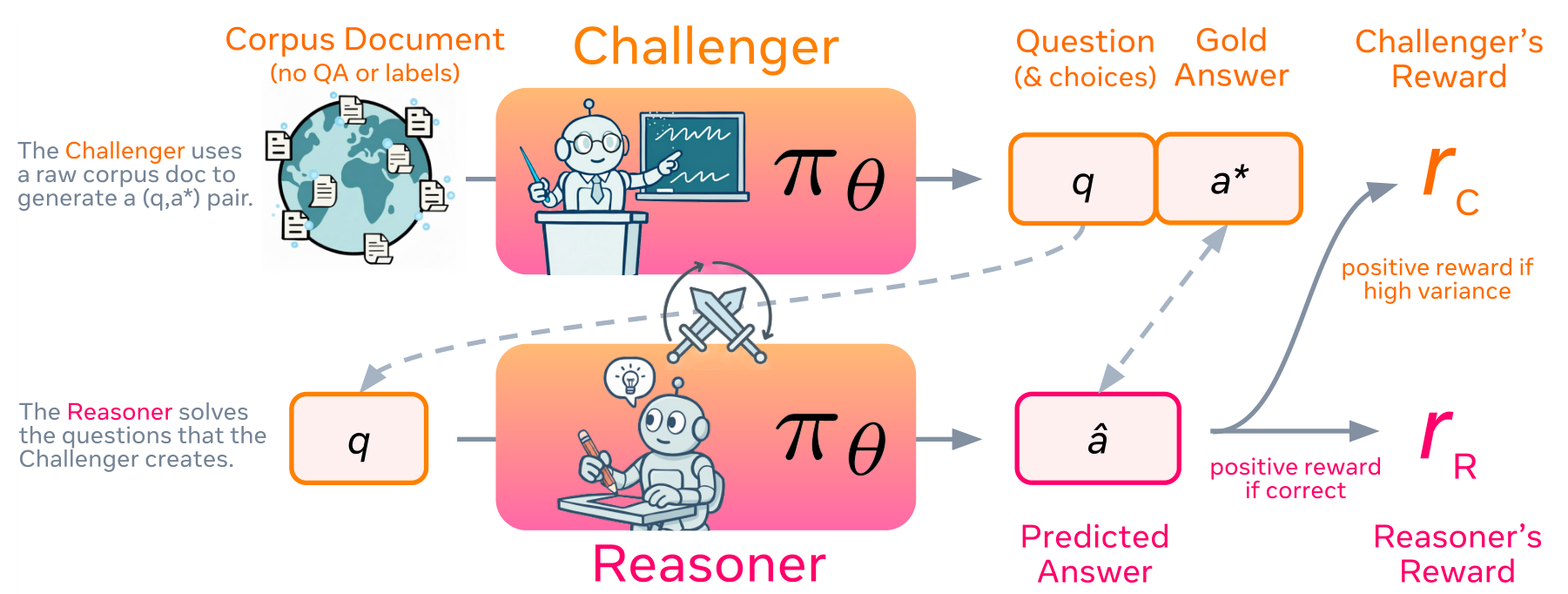
In SPICE (Self-Play In Corpus Environments), a single model acts as challenger and reasoner. The challenger reads an external corpus and uses a document to generate a question and reference answer. The reasoner answers without seeing the document. The two roles share weights but receive different information. SPICE, sections 2.1–2.3
This differs from the common RAG arrangement in which retrieved documents are provided during answering. Here the document informs the question and learning signal, and the solver must rely on its current abilities. External texts supply new material to a loop that might otherwise recycle only the model’s existing knowledge.
The paper generates multiple-choice and several short-answer formats. A rule-based verifier checks equivalence between the solution and the reference answer drawn from the document. The challenger earns high reward for questions with a useful mix of correct and incorrect attempts. The solver earns reward for matching the reference. The weights are shared, but the roles contribute learning signals from their respective rewards. SPICE, sections 2.2–2.4
External documents are essential to SPICE even when human involvement is reduced. They do not automatically make questions correct: the challenger may misinterpret a passage, write an ambiguous question, or extract the wrong answer. Documents provide a basis for verification while leaving room for generation errors.
#Supplement D — R-Few guides self-generation with a small pool of reference examples
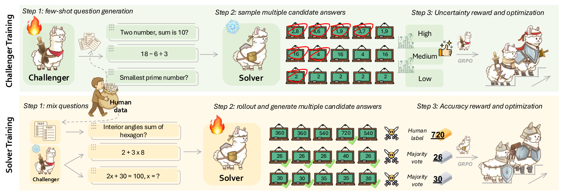
R-Few incorporates a small pool of labeled anchor examples into self-generation. The challenger samples some as in-context examples for creating new problems. The solver trains on both synthetic and anchor questions, using an online curriculum that selects items at an appropriate difficulty. R-Few, sections 3.2–3.3
The paper’s sample of zero to five examples refers to the context for a single generation call. The entire training procedure can use more than five human examples. In-context examples for generation and labeled training data for the solver are separate paths. R-Few, equation 4 and Algorithm 1
R-Few uses limited human information to keep self-generation on course. External references aim to reduce repetitive questions and drift from the desired task distribution. The paper also describes a short supervised fine-tuning (SFT) stage for output formatting. Even within a lecture on minimizing human involvement, the kinds of supervision that remain vary by method. R-Few, introduction and section 3.2
When reading the figure, distinguish the reference answer from the majority-vote answer. The paper identifies the problems as illustrations. For “2x+30=100” at the bottom, the true solution is 35. Three responses say 30 and two say 35, so the majority label reads 30. When mixing externally labeled examples with synthetic pseudo-labels, check which signal scores each item. R-Few, Figure 2
#How much trust does a verifier’s signal deserve?
Another study on slide 5, Self-Questioning Language Models, addresses this issue directly. For mathematics it uses a majority vote among sampled answers as a proxy for correctness. For coding it uses unit tests written by the proposer. The paper observes that there is no automatic reason to expect the proposer to be more accurate than the solver. Self-Questioning, section 4.2
The five approaches can now be compared by both the source of their problems and the origin of their correctness criterion.
| Method | Inputs for question generation | Main grading criterion | Open question |
|---|---|---|---|
| Absolute Zero | Model-generated code tasks and previous tasks | Results from code execution | Do the execution conditions and test coverage capture the intent? |
| R-Zero | Questions from the current model | Pseudo-label from multiple responses | Can the system detect a wrong but frequent answer? |
| Self-Questioning | A supplied topic and model-generated problems | Majority vote for math, generated tests for code | Could consensus and tests share the same error? |
| SPICE | An external document corpus | Equivalence to an answer extracted from the document | Do the question and answer accurately reflect the source? |
| R-Few | Synthetic problems and a small pool of anchors | Anchor ground truth and synthetic pseudo-labels | How are items with different sources of supervision selected and mixed? |
All these approaches start with pretrained models and human-designed training procedures. “Zero” and “Few” tell us little by themselves about the human knowledge embedded in the system. Specify whether the reduction concerns manual question writing, answer annotation, or human intervention during the loop.
#Worked example 3 — The same verifier produces different training data as input quality changes
Suppose a hypothetical verifier accepts 90% of correct answers and incorrectly accepts 10% of wrong ones. Let t be the conditional probability of accepting a correct answer, f the probability of accepting an incorrect answer, and p the fraction correct before verification. The fraction correct among accepted answers is:
The numerator is the fraction of all answers that are both correct and accepted. The denominator is the total fraction accepted, whether correct or incorrect. Assume t=0.9 and f=0.1 hold for both input populations. The following hypothetical groups have exactly those rates.
| Composition of 1,000 generated answers | Correct accepted | Incorrect accepted | Total accepted | Actual accuracy among accepted answers |
|---|---|---|---|---|
| 600 correct, 400 incorrect | 540 | 40 | 580 | 540/580 ≈ 93.1% |
| 200 correct, 800 incorrect | 180 | 80 | 260 | 180/260 ≈ 69.2% |
The verifier has the same conditional performance, yet lower-quality generated answers lead to more incorrect answers in the retained training data. Even the first group includes accepted errors. The claim “we trained only on verified data” therefore needs information on both verifier performance and the distributions before and after filtering.
In practice, t and f can also vary by problem type. If a generator and verifier share errors from a common base model, repeated mistakes may pass consistently. This example isolates one point: even with fixed conditional probabilities, acceptance rate and accuracy measure different things.
#Three connections to check in self-learning
First, the link between objective and problem. Proposer-generated tasks should exercise the intended skill. Solver uncertainty alone cannot tell us whether a question is clear or useful.
Second, the link between a solution and its verification. Execution results, majority votes, document-derived answers, and human anchors offer different grounds for trust. The learning signal depends on what was checked and which errors can still pass.
Third, the link between training and final evaluation. A higher internal reward or better performance on generated problems is observable. Whether that gain transfers to new tasks must be tested on data held out from selection, with comparable compute budgets.
The proposer–solver–verifier loop can reduce the need to write training material by hand. The source of new information, the criterion for rejecting incorrect answers, and its alignment with the actual goal determine the nature of the improvement. As the second lecture continues, track both what the model changed and what that change achieved.
Part 15 turns to improving the harness itself. Starting with the human design behind prompts for generating problems, it examines ways to change prompts, tools, and workflows while keeping weights fixed, and how to compare the results.
Calculations and code
The code calculates the gradient step on a hypothetical loss, AZR’s base rewards, R-Zero’s agreement, difficulty, and repetition penalties, the incorrect modal answer, and accuracy before and after verification. It checks the quadratic gradient by central differences, the triangular reward against its piecewise expression, and verifier probabilities against an item-level confusion matrix. It illustrates the calculations without training the papers’ models or reproducing their benchmarks.
#Further reading
| Resource | Relevant topic |
|---|---|
| NTU second lecture · Slides 1–5 | Objectives, training loss, evaluation, and the proposer, solver, and verifier |
| Lambert L9 — Over-Optimization · Slide 8 | Overfitting, proxy overoptimization, and metric mismatch on validation data |
| Lambert L7 — Synthetic Data · Slide 7 | Synthetic questions, responses, and grading signals across the three roles |
| CMU L9 — RL Foundations for Agents · Slide 41 | Difficulty and the loss of group-relative learning signals under equal rewards |
| Absolute Zero: Reinforced Self-play Reasoning with Zero Data | Executable tasks and environment-based rewards |
| R-Zero: Self-Evolving Reasoning LLM from Zero Data | Alternating challenger and solver training with pseudo-labels |
| Self-Questioning Language Models | Question generation, majority votes, and generated unit tests |
| SPICE: Self-Play In Corpus Environments Improves Reasoning | Document-grounded question generation and asymmetric information |
| Guided Self-Evolving LLMs with Minimal Human Supervision | R-Few’s limited example supervision and mixed curriculum |