Getting the right loss on average and updating parameters in the right direction are different things. If the model determines the distribution that supplies the samples, its derivative also matters.
Part 7 — When should self-training stop, and when should a model adapt? distinguished the scope of self-training from test-time training. Here we examine the calculation behind entropy minimization. Does the expression we actually backpropagate give the gradient of the entropy we want to reduce?
Video timestamps by slide
| Slide | Video segment and topic | Related concept |
|---|---|---|
| 36 | 36:00–36:33 — Introducing the math and the study | Loss values and gradients, notation and assumptions |
| 37 | 36:33–39:55 — Sequence and token entropy and their relationship in expectation | Chain rule and a two-token probability tree |
| 38 | 39:55–41:11 — Computing a gradient with the sample held fixed | Changes to the sampling distribution versus automatic differentiation |
| 39 | 41:11–42:44 — The missing term in the derivative of an expectation | Product rule, log-derivative identity and a correction to the slide |
| 40 | 42:44–43:24 — Reducing entropy along the selected path | Gradient sign, numerical counterexample and a surrogate loss for implementation |
#Slide 36 — Does equality of values imply equality of gradients?
In the video · 36:00–36:33. The lecturer asks how entropy can serve as a loss when enumerating every possible answer is impractical. He introduces research from his lab and turns to the mathematics.
Rethinking Entropy Minimization in Test-Time Adaptation for Autoregressive Models explains entropy minimization for autoregressive models in terms of two gradient components. Huang et al., arXiv v1
#Further reading A — Why do two losses appear together?
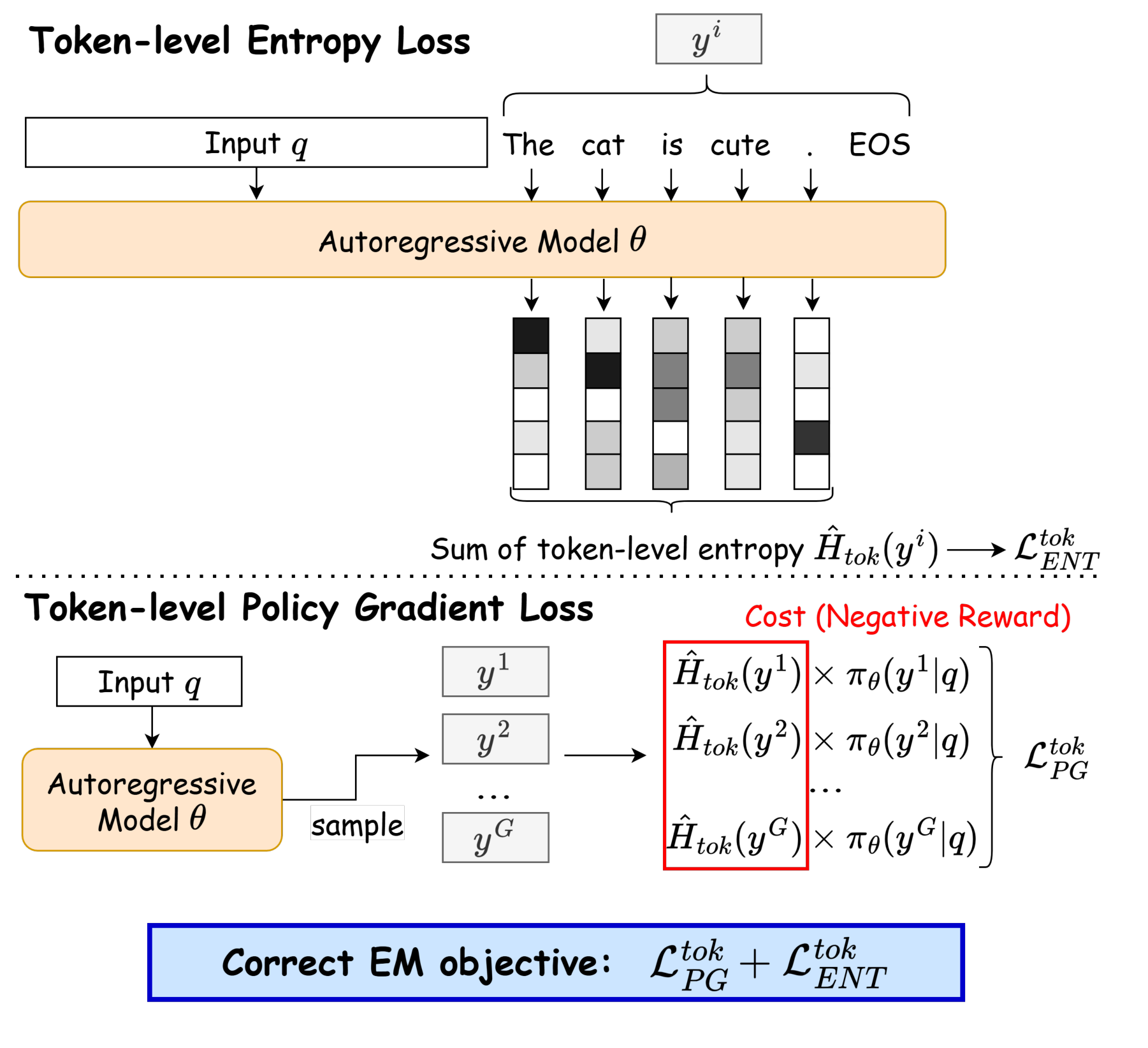
The upper half reads a given token sequence as context and sharpens the distribution at each position. The lower half generates several output paths and trains the model to select paths with lower costs more often. The arrows and multiplication signs are schematic. Use the exact derivatives in the paper when implementing them. Figure 1 and equations (8)–(9)
Keep four questions distinct as you read these five slides.
| Quantity | Question |
|---|---|
| Objective value | What is the entropy over all answers the model can produce? |
| Sample estimate | How can one generated answer estimate that quantity? |
| Fixed-sample gradient | What do we get if we fix the sampled tokens and differentiate the loss? |
| Full objective gradient | Have we included the effect of sampling different answers as the parameters change? |
We use for the input, for the random token sequence and for one sampled sequence. is the probability that the model generates that sequence. We use natural logarithms and measure entropy in nats.
We start with a fixed finite length and a finite vocabulary. We can then sum over all outputs and check the derivatives directly if the probabilities are positive and differentiable. Variable-length sequences with an end-of-sequence token (EOS) require additional conditions, discussed at the end of slide 37.
#Slide 37 — Computing sequence entropy one token at a time
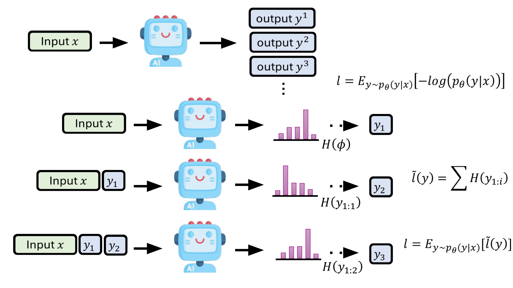
In the video · 36:33–39:55. The lecturer contrasts a classifier’s finite outputs with the large output space of text generation. He calculates the next-token distribution and sums the token entropies along a generated path. The relationship between the expectation of this sum and full entropy is our starting point.
#What exactly is infeasible to compute?
With vocabulary size V and length T, there are V to the power T possible sequences of fixed length. Entropy is well defined. What becomes impractical for a large model is enumerating all sequences exactly. In a small model, we can list every output and calculate entropy directly.
The entropy of the full output is
An autoregressive model assigns a probability equal to the product of token probabilities conditioned on the preceding tokens.
Turning this product into a sum does not imply that the tokens are independent. It follows from the chain rule for conditional probabilities. Different preceding tokens can give different distributions for later tokens.
#H on the slide describes a distribution before the token is selected
Given a prefix s, calculate entropy over the whole next-token distribution.
The slide’s corresponds to the initial empty prefix. The H terms below it use prefixes containing previously sampled tokens. Here we denote the empty prefix by . Having already selected A does not set this entropy to zero. We are evaluating the distribution before choosing the next token in that context.
Define the sum of entropies over the prefixes visited on one path as follows. It corresponds to the slide’s surrogate loss, with a subscript to show its dependence on the parameters.
This value generally differs from the negative log probability of that path. Their expectations coincide when we sample paths from the model’s own distribution.
This is unbiasedness of the value estimate. Averaging over many paths drawn from the same distribution estimates the full entropy. Neither the value on a single path nor its derivative must equal the full entropy or its gradient, respectively. Paper §3.1, equations (3)–(7)
#Further reading B — The chain rule uses conditional entropy
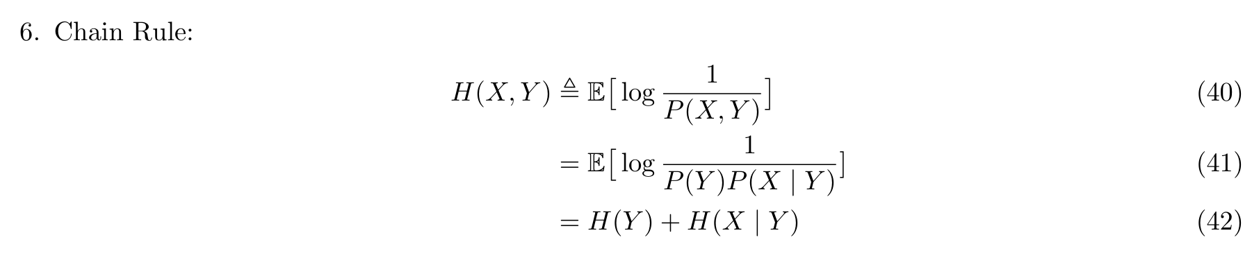
The Stanford notes decompose the joint entropy of two random variables into the entropy of one and the conditional entropy of the other. Conditional entropy also averages over the possible values of the conditioning variable. The notes use base-2 logarithms by default. The identity is the same with natural logarithms, but converting the numerical values requires a change of units. Definitions and logarithm base · Chain rule
#Worked example — A small model with four possible answers
Consider a model that generates two tokens. The first is A or B with probability 0.5 each. After A it generates 0 or 1 with probabilities 0.9 and 0.1. After B the two probabilities are 0.5 each. After two tokens it terminates with probability 1, so termination contributes no further entropy.
| Output path | Path probability | Sum g of entropies of the token distributions visited |
|---|---|---|
| A0 | 0.45 | 1.018230 nat |
| A1 | 0.05 | 1.018230 nat |
| B0 | 0.25 | 1.386294 nat |
| B1 | 0.25 | 1.386294 nat |
Writing h for binary entropy gives
Computing the full entropy directly from the probabilities of the four paths gives the same result.
For the single path A0, g is 1.018230, while the full entropy is 1.202262. Greedy decoding always picks the most likely path A0 here and therefore cannot stand in for the expectation under the original distribution.
Conditions for variable length. The paper proves unbiasedness of the token estimator for finite sequences ending in EOS when the entropy is finite. An implementation should include EOS and exclude subsequent padding. Truncation at a maximum length or averaging by token count can change the objective. Also, the conditions for an unbiased value do not by themselves justify exchanging differentiation and an infinite sum. We first derive the gradient for a fixed, finite output space. Theorem 1 and proof
#Slide 38 — What does differentiating with a fixed sample leave out?
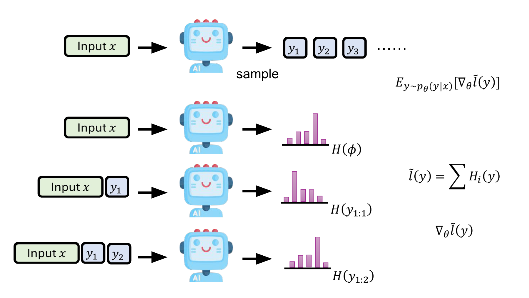
In the video · 39:55–41:11. The lecturer first samples a token sequence and feeds its prefixes back into the model to compute the token entropy gradients. A different path is sampled each time, so the average update is expressed as an expectation.
The bottom of the figure feeds previously sampled tokens in as input. Automatic differentiation treats these token IDs as fixed. It differentiates the logits, probabilities and entropy with respect to the parameters given those tokens as context.
The resulting gradient for one sample is
Let A be the average of this gradient over samples.
The gradient of the actual objective, however, is
The two expressions appear to differ only in the position of the gradient. The important difference is that the distribution defining the expectation also depends on the same parameters. A weight change alters both the entropy at a given prefix and the probability of reaching it.
The expectation contains the product of two parameter-dependent terms.
More samples can reduce the sampling error in estimating A. Even a perfect estimate of A still omits part of the full gradient. Repeating the calculation cannot remove the bias from the missing term.
Discrete sampling does not preclude computing the gradient. Instead of differentiating the sampled ID directly, we can use the gradient of its selection probability. The log-derivative identity in the next section gives the connection.
#Slide 39 — The product rule gives two terms
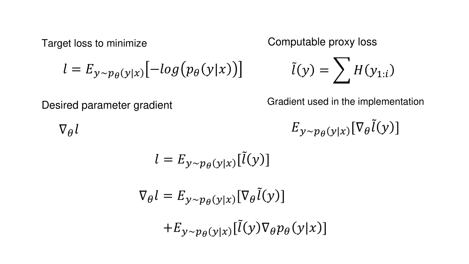
In the video · 41:11–42:44. The lecturer emphasizes that although the computable surrogate loss equals the objective in expectation, moving the derivative inside the expectation can drop a term.
#Deriving the gradient line by line
In our finite output space, assume positive, differentiable probabilities and fix the input x. Start with the product rule.
The first sum already weights each term by its probability and is therefore an expectation. To turn the second sum into an expectation under the same distribution, multiply and divide by the probability.
The exact decomposition is
A directly changes the cost of a visited path. B changes how often different paths are selected. Interpreting cost as negative reward connects B to the policy gradient. The decomposition follows by applying the product rule to the equality of values. Equation (8f) of the paper likewise contains the gradient of the log probability. Paper, PDF p. 3
#A notation trap — ∇p in the sum, ∇log p in the expectation
The final term in the original image takes the following form.
This form is incorrect in general. The gradient of the probability belongs in the sum without probability weights. To express the same term as an expectation under p, use the gradient of the log probability.
The expectations on slides 39 and 40 omit log. Use the log-probability gradient as on the right side of the identity above.
#Further reading C — Berkeley’s log-derivative identity
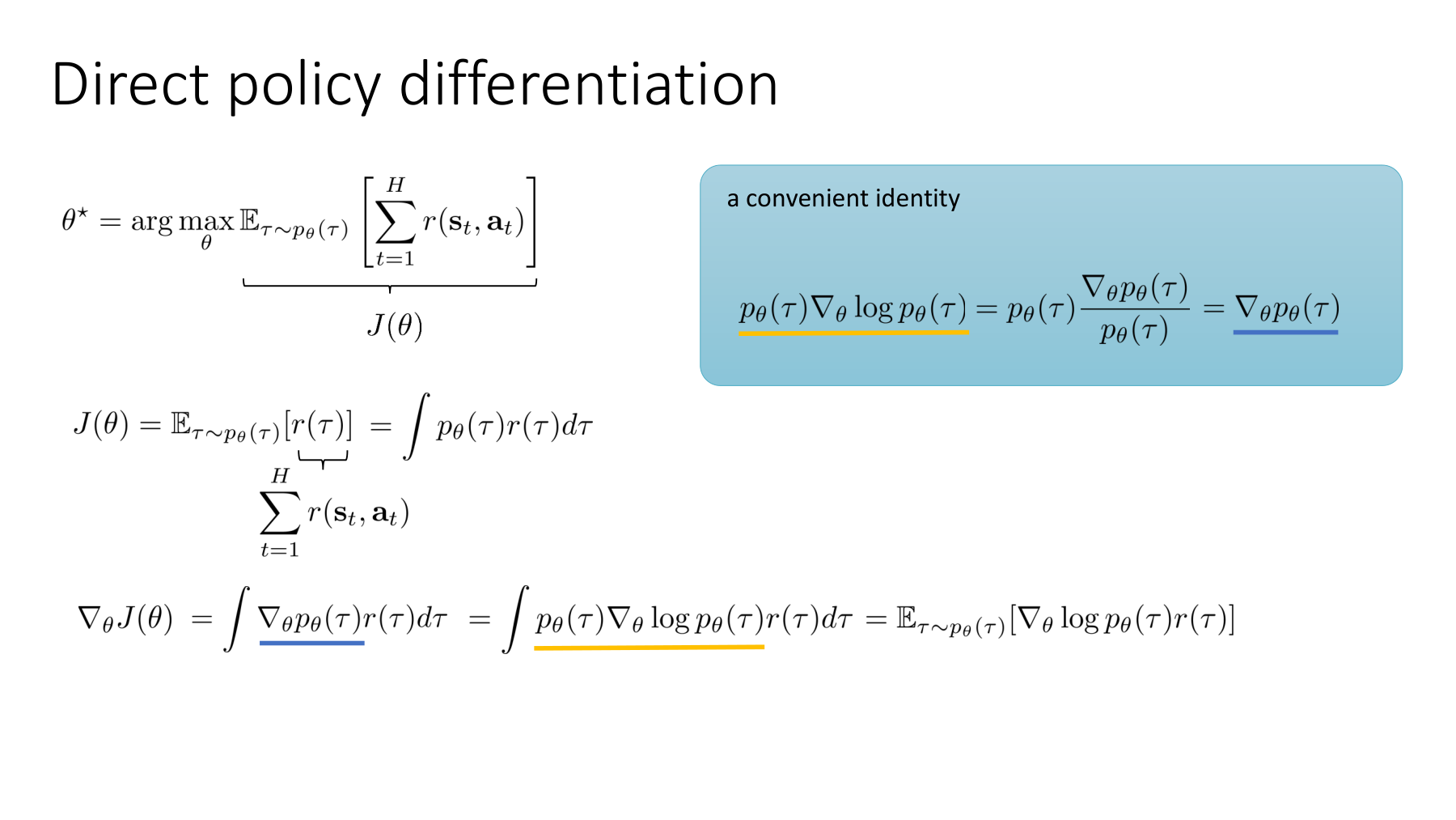
The equation in the blue box is the log-derivative trick we just used. Berkeley maximizes reward, whereas here we minimize an entropy cost. Mixing the signs for reward and cost reverses the update direction. Also, unlike the reward in the diagram, g here depends directly on the parameters. We must retain A as well as B. Original PDF, p. 5
#A probability tree with a correct value estimate and a zero gradient
Return to the two-token model on slide 37. This time only q, the probability of A as the first token, can change. Keep 0.9 after A and 0.5 after B fixed. Let q be the sigmoid of a logit z.
The exact derivative is
At q = 0.5 the entropy gradient of the first token itself is zero. But the distribution after A has lower entropy than the one after B. This difference contributes to the full gradient.
| Calculation | Gradient with respect to z | Effect of gradient descent |
|---|---|---|
| Differentiate full entropy over all four paths | −0.092016 | Increases z, making A more likely |
| Use only the fixed-sample token entropy gradient A | 0 | Cannot change the first branch probability |
| Include both A and the correct B | −0.092016 | Matches the derivative of full entropy |
| Use the slide’s expectation term without the logarithm | +0.017725 | Moves the first branch in the opposite direction in this example |
These are exact calculations over all four paths. The positive sign in the last row is not a rounding artifact. Using the probability gradient inside an expectation already weighted by p changes the weights. A finite-difference check of the full objective also gives −0.092016.
Limit of this interpretation. The model does not specify whether answers on path A are factually correct. This calculation determines the entropy gradient’s direction. Improving accuracy is a separate question. As Part 6 noted, a model can become more confident in an incorrect answer.
#Slide 40 — Making the selected path more certain
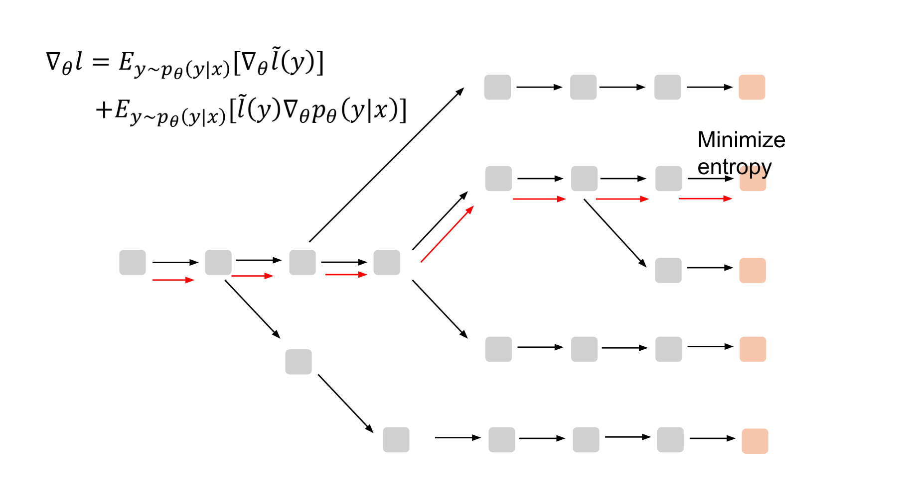
In the video · 42:44–43:24. With a diagram of branching token paths, the lecturer explains the term that reduces entropy on the selected path. Slide 41 turns to changes in the probability of selecting other paths.
The red arrows mark the path used for the calculation. They do not identify a correct answer. A gives a gradient that sharpens distributions at fixed prefixes. On its own it does not account for the selection probabilities of all paths.
The slide speaks of the gradient as an update direction. When minimizing, parameters actually move in the negative gradient direction.
#How does token entropy change the logits?
For a given context, write z for the logit vector and p for the softmax probabilities. The derivative of token entropy with respect to each logit is
Because probabilities are normalized, each logit affects the other probabilities too. The gradient is zero at a uniform distribution. Reducing entropy therefore need not strengthen the best answer. This also explains why A cannot change the first branch in our probability tree when the initial distribution is exactly 0.5 versus 0.5.
#Further reading D — Building a surrogate loss for automatic differentiation
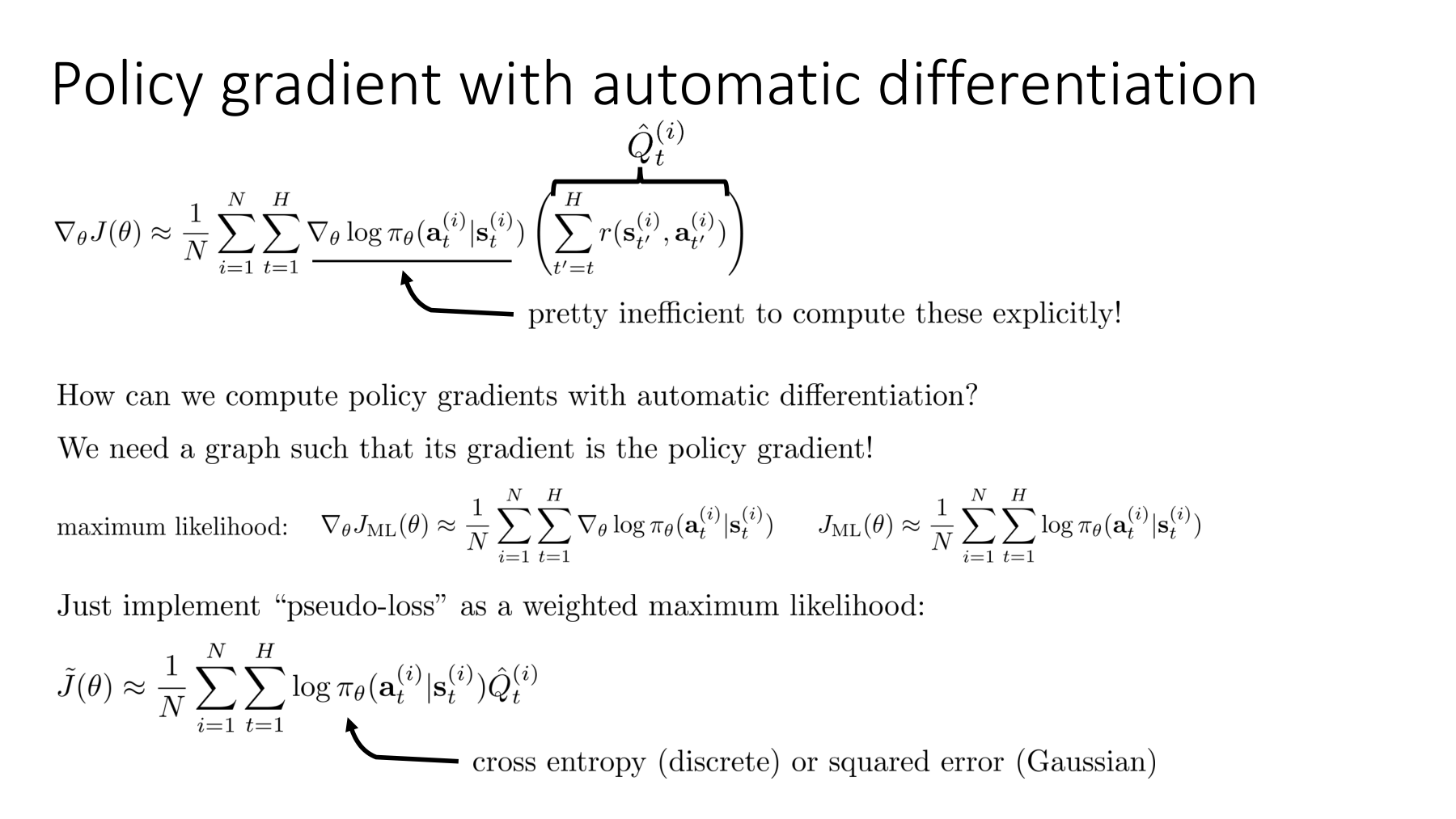
The slide builds the computation graph to produce the gradient we want. The surrogate loss passed to backpropagation can have a different numerical value from the original evaluation metric. Its purpose is to give the required gradient estimate when differentiated. Berkeley PDF, p. 20
Hold the sample y fixed during differentiation. Write sg for stop-gradient, which preserves a value but blocks differentiation along that route. The implementation loss corresponding to equation (9) is
Here b is a fixed baseline independent of the sampled answer. Start with zero. Differentiating one sample gives
The baseline leaves the expected gradient unchanged because the probabilities sum to one.
Substituting a batch mean that includes the current sample, however, can make the baseline depend on that sample. Claiming unbiasedness then requires a separate design or correction. The code below uses a fixed scalar baseline.
#The essential PyTorch calculation
The excerpt below is the core of a function that validates input shapes, data types and masks. logits contains logits recomputed at each sampled prefix, sampled_tokens contains the sampled token IDs, and valid_mask is true through EOS and false for padding.
# logits: [batch, time, vocabulary]
# sampled_tokens: [batch, time], dtype=torch.long
# valid_mask: [batch, time], dtype=torch.bool
logp = torch.nn.functional.log_softmax(logits, dim=-1)
token_entropy = -(logp.exp() * logp).sum(dim=-1)
token_logp = logp.gather(-1, sampled_tokens.unsqueeze(-1)).squeeze(-1)

entropy_sum = (token_entropy * valid_mask).sum(dim=1)
sequence_logp = (token_logp * valid_mask).sum(dim=1)
loss = (entropy_sum + (entropy_sum.detach() - baseline) * sequence_logp).mean()
detach() makes the cost in the second term act only as a weight. Omitting detach there introduces an extra derivative of the cost multiplied by the log probability. Detaching the first entropy_sum as well would remove A. The signs here assume cost minimization. Equation (9) · PyTorch detach documentation · log_softmax documentation
If the function returns one loss per sequence, the caller should take the mean before backpropagating.
Implementation conditions. The policy that generates samples must match the distribution used in the loss. Arbitrary top-k or top-p filters, different temperatures, or samples from a stale model can invalidate the unbiasedness claim. Keep the model fixed between sampling and recomputation and handle stochastic behavior such as dropout consistently. model.eval() disables dropout. no_grad() separately disables gradient tracking.
Keep input prompt tokens separate from generated answer tokens and sum only over the generated portion, including EOS. Averaging by length can change the objective. Low-precision probabilities can be numerically unstable, so the full function performs the calculation in float32 for half and bfloat16 logits. These checks clarify the conditions of the calculation. Accuracy and stable adaptation still require evaluation.
#What these five slides establish
Under appropriate sampling conditions, the sum of token entropies can be an unbiased estimate of sequence entropy. Differentiating only that sum with the sample held fixed can omit changes in the distribution that selects the path.Both terms on slide 39 follow from one objective. Differentiating the expectation accounts for changes to the cost and to the probabilities. Even the missing logarithm on the original slide can reverse the gradient direction, as the worked example shows. Checking the equations, the implementation and a small numerical example together catches this error.
Part 9 — The gradient that selects paths and a model that makes its own training problems continues with slides 41–45. We examine the path-selection term, comparison conditions in a speech recognition results table, AI evaluation and input generation.
#Further reading
| Resource | Where to look | Connection |
|---|---|---|
| NTU lecture video, first half | 36:00–43:24 | Entropy estimation and the two gradient terms |
| NTU Self-Improving PDF | Slides 36–40 | Entropy values and gradients |
| Huang et al., arXiv:2605.08186v1 | Figure 1, §3.1–3.2, equations (3)–(9) | Estimator conditions, exact gradient and stop-gradient |
| Stanford EE376A lecture notes | Lecture 3, January 16, 2018, pp. 1, 5 | Entropy units and the chain rule |
| Berkeley CS 185/285 lecture slides | PDF pp. 5, 20 | Log-derivative identity and an autodiff surrogate loss |
Code and numerical checks
The 30 numerical checks and eight PyTorch autograd checks enumerate all four paths to compare entropy, gradients and baselines. The full function with shape, data type and mask handling documents its input requirements.