A reward that is easy to learn from can differ from the goal we want to achieve. Even when AI designs the reward, evaluate the policy trained on it using a separate success criterion.
Part 3 distinguished self-correction, which revises an answer, from training, which changes model parameters. It also compared supervised imitation of a target with reinforcement learning from rewards.
That leads to the next question. If we can give a score instead of a correct answer, who should design that score, and how?
#Slide 16 — Success is clearly defined but rarely encountered
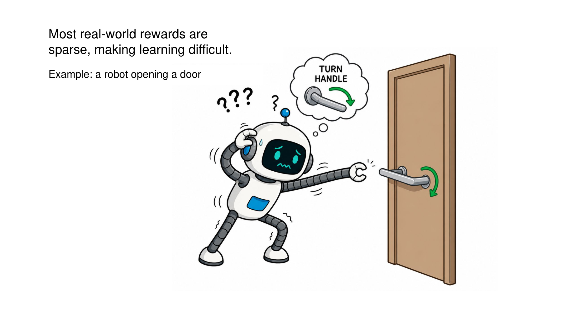
The slide raises the problem of sparse rewards in practice, using a robot opening a door as an example.
Suppose the task gives one point only when the door opens and zero otherwise. The following is a simplified illustration, separate from actual robot reward code.
The success criterion is clear. But if an unskilled policy repeatedly fails to open the door, every observed task reward is zero. A trial that approaches the handle can receive the same score as one moving in the opposite direction.
What is missing is a learning signal indicating which attempts came closer to success. When exploration rarely encounters useful experience, there are fewer opportunities to learn from it.
A zero reward does not imply that all learning must stop. Depending on the algorithm, value estimates, entropy terms, pretraining, or separate exploration signals may contribute. The difficulty is that the task’s success reward alone provides little basis for distinguishing better actions.
#Calculating sparsity with a 0.1% chance of success
For a toy calculation, assume that training has yet to change the policy, that trials are independent, and that each has a fixed success probability of 0.001.
The probability of at least one success in 100 trials is
Even after 100 attempts, the chance of experiencing success at least once is only about 9.52%. The expected number of trials to first success is
In actual RL the policy changes, and trials may be correlated. These figures give neither a prediction nor a lower bound for robot training sample requirements. They illustrate how obtaining successful experience can itself become the bottleneck when reward events are rare.
#Further reading A — Sparse and dense rewards at UMass
Scott Niekum, CS 690 Reward Specification, PDF page 4
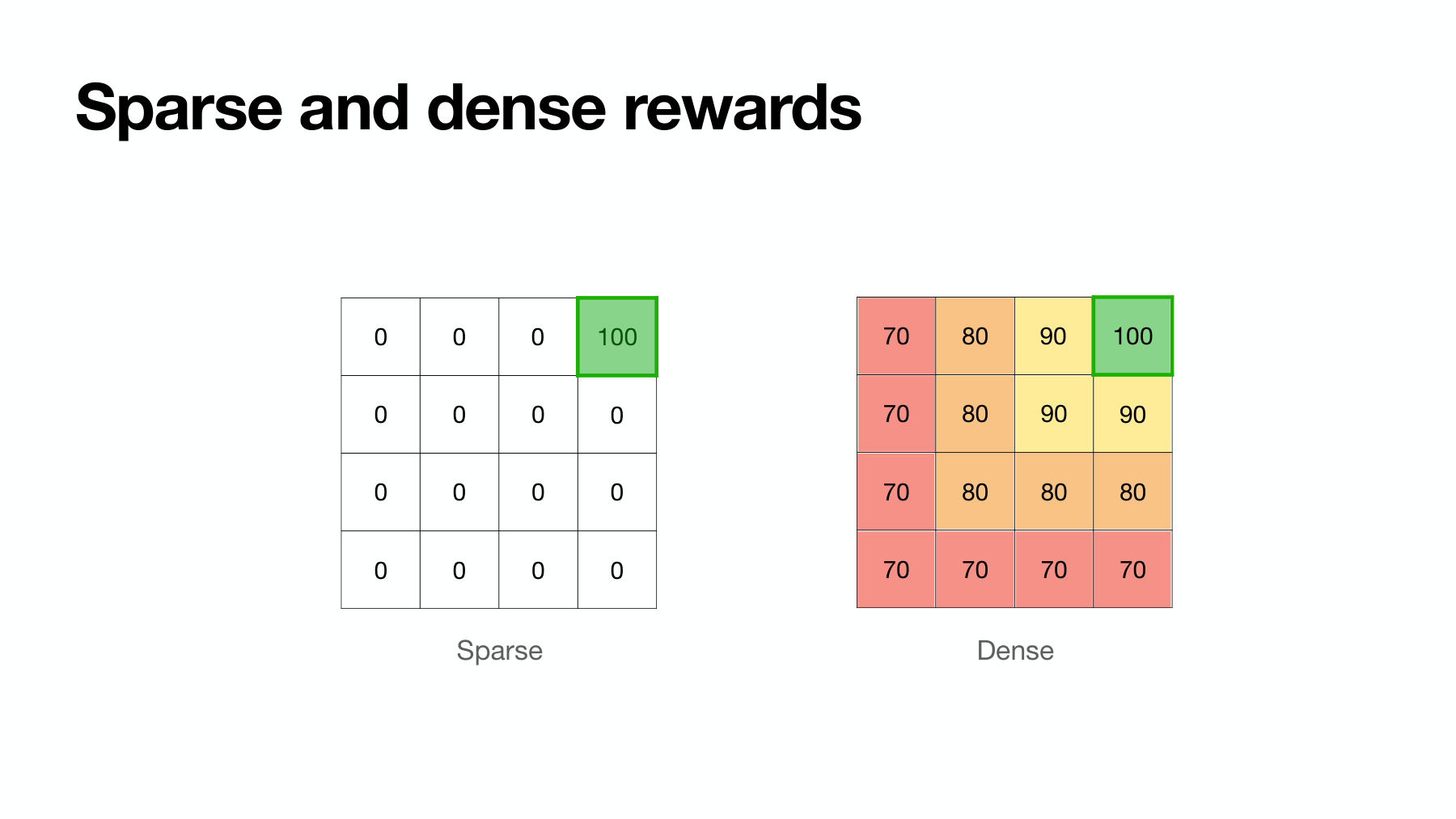
The lecture slide compares a grid with a large value only at the goal against one with values at multiple locations. The left grid represents a simple success condition. The right distinguishes more situations along the way.
Separate observing informative values more frequently from the claim that actions maximizing them best serve the original goal. Dense rewards provide more learning signals, but adding signals alone does not preserve the objective.
Sparse and delayed rewards are also distinct. Sparsity concerns how infrequently a reward event occurs. Delay concerns time between an important action and its consequence. Door opening can exhibit both.
#Slide 17 — Break door opening into steps and keep the ultimate goal in view
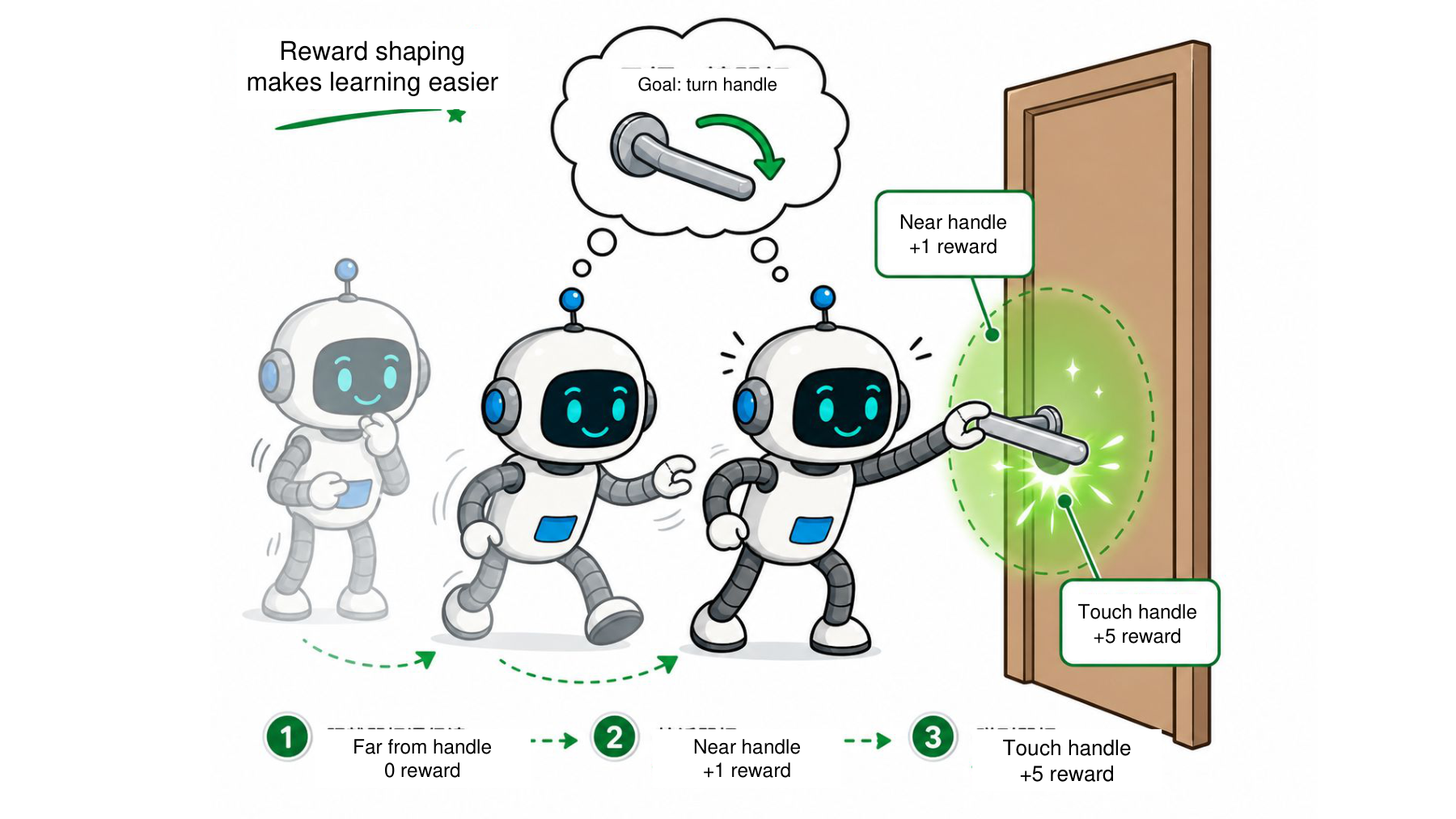
Slide 17 assigns zero far from the handle, +1 when approaching, and +5 for contact. These are different illustrative reward settings from the +0.5 for contact and +1 for opening on slide 18.
Given the goal “open the door,” a researcher might consider the following intermediate events.
| Stage | Observable change | What it leaves uncertain |
|---|---|---|
| Approach | Fingertip-to-handle distance decreases. | Suitable hand orientation and collision avoidance need separate checks. |
| Contact and grasp | The robot touches and grasps the handle. | The handle may not have turned and the door may still be closed. |
| Manipulate the handle | Handle angle or latch state changes. | Door motion and eventual passage are separate outcomes. |
| Move the door | The opening angle increases. | The target angle, duration, and safety conditions need verification. |
The table helps identify measurable signals before final success. It does not prescribe one sequence for all doors. A handleless door, a push door, and an automatic door have different intermediate steps.
#State, action, and reward have different roles
State can include task information such as hand position, handle angle, and door angle. Actions depend on the control interface, such as target joint positions or force commands. A reward is a number evaluating the state, action, and next state.
For simplicity, the expression below assumes a fully observable Markov decision process (MDP).
An actual camera-based robot uses observations without direct access to the full state. Estimating these state variables from video is a separate problem. Reward design does not automatically resolve perception error or sensor delay.
#What changes when intermediate events receive rewards?
Adding a term for proximity to the handle distinguishes actions even before the first successful opening. Designing auxiliary rewards to aid learning is the basic idea of reward shaping. Ng, Harada, and Russell, section 2.2 also describes adding an auxiliary term to the original reward.
If approaching becomes the effective objective, the robot may stop at the door. A large reward for grasping may encourage holding the handle indefinitely. A good intermediate signal helps the policy learn actions leading to final success within a limited training budget.
#Slide 18 — Even an AI-designed reward can change the objective
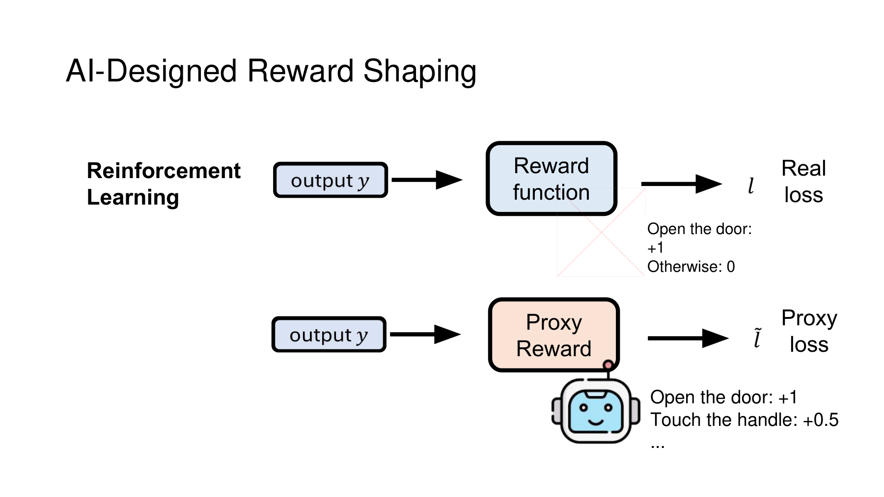
The slide distinguishes the original reward function from a proxy reward. The example scores successful door opening under the original goal and adds an intermediate signal such as handle contact to the proxy.
Reinforcement learning generally concerns return accumulated across time steps. The difference between an instantaneous score and return creates a reward design pitfall.
The discount factor determines the weight of future rewards relative to current ones. is the maximum trajectory length considered here.
#A counterexample — Collecting contact points without opening the door
Consider a hypothetical thought experiment in which the +0.5 contact reward can be collected repeatedly.
Start in a state where the door can be opened immediately. Opening it earns one point and ends the episode on that step. If the door stays closed but the robot touches the handle, it earns 0.5 per step. The horizon is 20 steps and the discount factor is 0.99.
Policy A maintains contact for 20 steps without opening the door. Policy B opens it on the first step and terminates. The example does not award contact and success together.
| Policy | Actual opening | Return under the designed reward |
|---|---|---|
| A: maintain contact | Failure | About 9.10 |
| B: open immediately and terminate | Success | 1.00 |
The reward ranks sustained contact above the intended success. The agent has calculated the score correctly. Behavior that faithfully maximizes the designed score has diverged from the behavior we wanted.
Paying once on first contact can reduce this particular form of repeated collection. Other shortcuts may still change the effective objective, for example rushing to an intermediate milestone and then abandoning the task.
#Further reading B — Potential-based reward shaping
Scott Niekum, CS 690 Reward Specification, PDF page 5
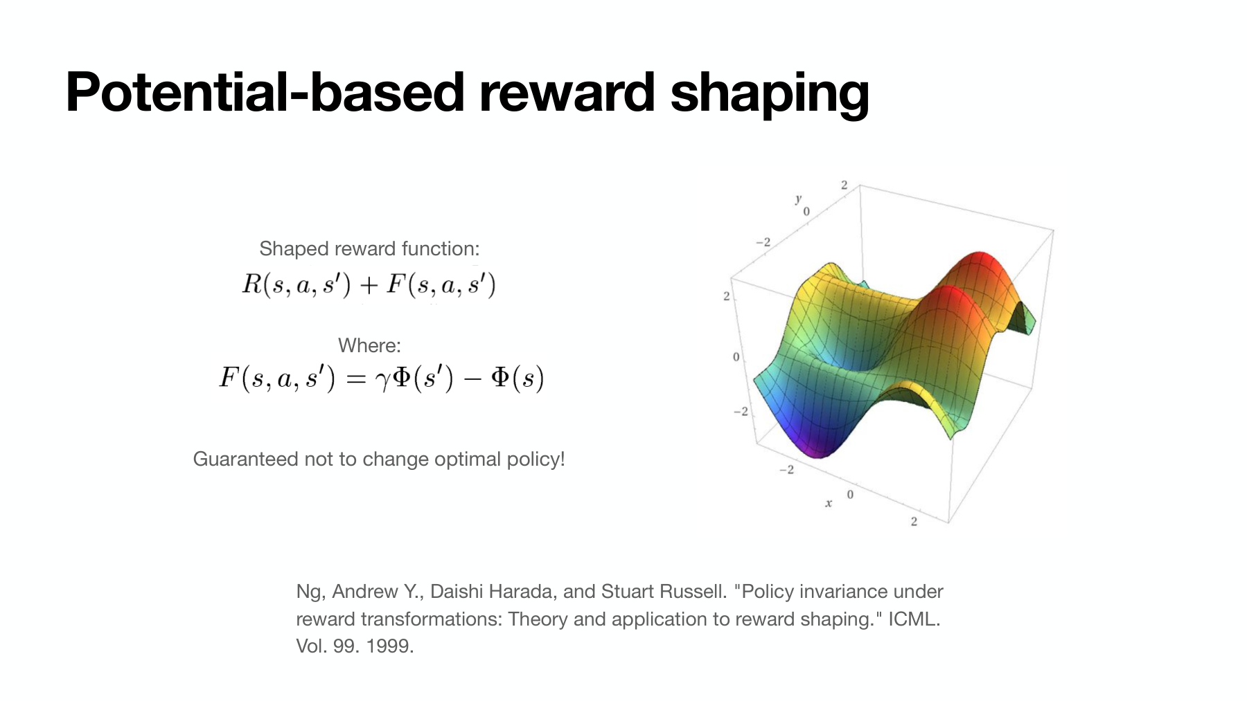
We can add a term whose structure permits analysis of policy preservation. Potential-based reward shaping (PBRS) uses differences in a potential function defined on states.
Theorem 1 in Ng, Harada, and Russell (1999) studies how this transformation relates to preservation of optimal policies. The potential need not equal the true value function. The discount, state definition, and treatment of termination must meet the mathematical conditions before drawing a preservation claim.
Summing reward over a finite trajectory makes the intermediate potential terms cancel.
With the same initial state and terminal potential set to zero, the only added value is , independent of policy. The ranking of policies by return is preserved under these conditions. For an infinite discounted horizon, the same intuition follows as the boundary term vanishes when the potential is bounded and .
Conversely, truncating at a time limit while leaving an arbitrary final potential can make policy dependent. Distinguish actual termination from truncation by a time limit. For a finite horizon, also check the time-augmented state and potential and the final boundary condition.
#Numerical check — Intermediate rewards without changing the ranking
Assign the following potentials and original rewards to four illustrative states. The potentials are chosen to check the derivation and are not experimental estimates.
The added rewards are 0.46, 0.42, and 0.20, respectively. The training rewards therefore become
The difference is exactly . This single trajectory does not verify every policy. Rank preservation for all policies follows from the structure and boundary conditions above.
Moreover, preserving optimal policies does not guarantee faster learning. With finite samples, function approximation, exploration, and optimizer choices, learning outcomes require measurement. Check that an LLM-written reward actually has the required form before claiming PBRS guarantees.
#Slide 19 — Separate scores for training from criteria for evaluation
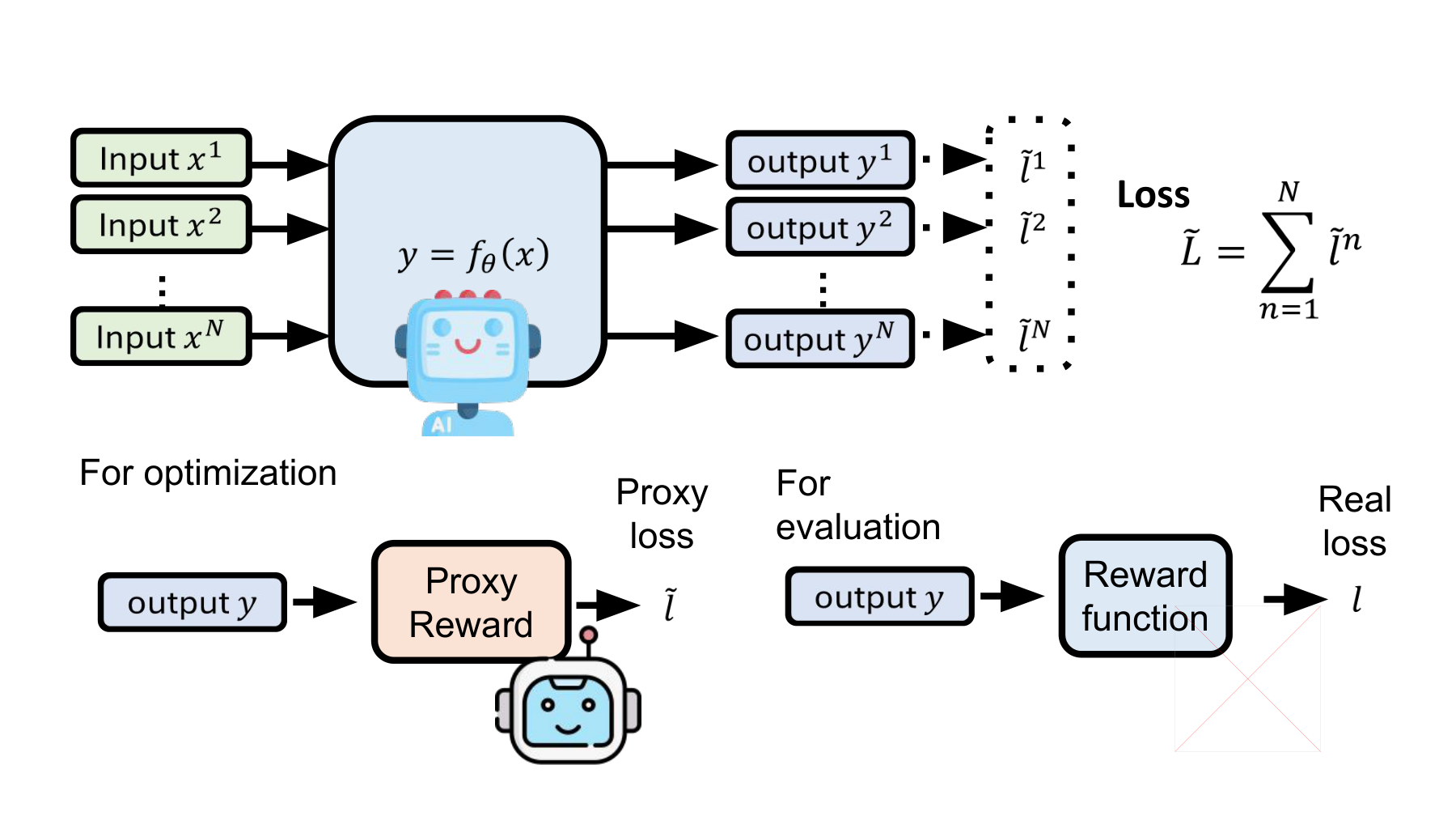
This slide distinguishes “For evaluation” from “For optimization.” Applied to the counterexample:
Training proxy reward: Provide useful signals during learning, such as approach, contact, and handle manipulation.
Separate task evaluation: Check whether the door actually opens, measure the success rate, and characterize failures.
The original also calls these quantities real loss and proxy loss. Rewards are maximized and losses minimized, but an implemented RL policy loss need not simply negate the numeric reward. Policy gradients, value estimates, and regularization may enter the training equation.
#Why raw scores from different reward candidates are incomparable
A new reward function may change units and scale. If one candidate awards 0.1 for approaching the handle and another awards 100 for the same event, their training-curve heights cannot be compared directly.
Multiplying the same reward by a positive constant of 100 multiplies raw return by 100 without multiplying actual success rate by 100. Even when the mathematical ranking is preserved, scale may affect training stability in practice. Include it among experimental conditions.
Compare reward candidates by what policies trained with them achieve under a shared evaluation criterion. A large number emitted by the reward conveys little on its own.
#Further reading C — Rewards can overfit to the training environment
Scott Niekum, CS 690 Reward Specification, PDF page 11
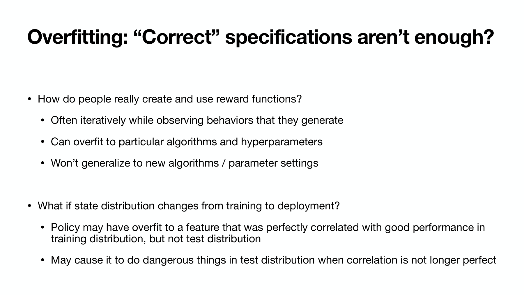
This supplementary slide considers overfitting as people repeatedly adjust rewards after observing training. The associated AAAI 2023 paper by Booth and colleagues investigates how trial-and-error reward design can overfit a learning algorithm and its settings or misspecify the intended task.
In our example, a reward working on one door and one initial pose cannot yet be generalized to door opening. Other handle positions, starting poses, or training settings may produce different results. The following design can reduce that risk.
| Stage | Data or settings | Appropriate use | Misleading use |
|---|---|---|---|
| Policy training | Training environments and initial states | Train a policy under each candidate reward. | Report the training score as independent final performance. |
| Reward candidate selection | Separate selection environments and seeds | Compare rewards and decide the next change. | Call a repeatedly consulted selection score an untouched test score. |
| Final evaluation | Conditions unused for candidate selection | Evaluate generalization after selection ends. | Revise the reward after inspecting the test and report that same result as final. |
Control training steps, compute, policy architecture, initialization, and evaluation seeds as far as possible. Report variation across seeds. The appropriate statistic and sample size depend on the experiment. No one run count is universally sufficient.
On real robots, monitor collisions, excessive contact forces, and joint-limit violations in addition to success. Penalizing an event does not establish that safety requirements are met. The experimental suggestion here is to validate with independent constraints and stopping mechanisms in place.
#Slide 20 — The LLM edits reward code, and evaluation measures the trained policy
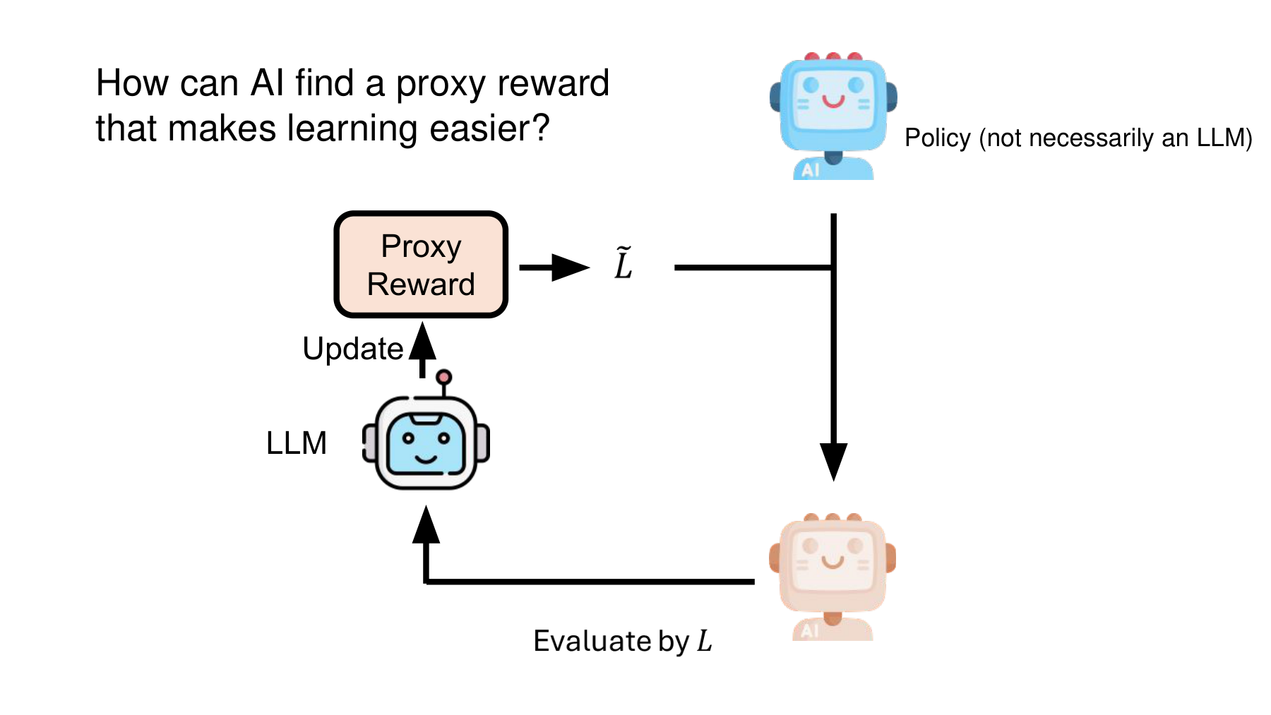
This slide asks how AI can discover which proxy rewards help learning. It also points out that the policy need not be an LLM.
There are two roles. The reward designer produces a reward function or code. The policy learner learns how to act in an environment using that reward. An LLM designer does not imply that the robot’s low-level control policy uses an LLM.
#Inner and outer loops
The inner loop holds a reward fixed and trains a policy. The outer loop revises candidate rewards based on the trained policy’s performance and failures.
We can express the two roles schematically as follows.
denotes a reward candidate’s code or settings, the policy parameters, and a fixed training budget. The outer objective is a good evaluation outcome for the policy trained with that reward. The size of the reward’s raw output is incidental.
The notation does not require differentiating the outer loop. An LLM can search by proposing code candidates, receiving textual feedback on actual training, and producing another candidate. Modifying code and training the LLM’s weights are different operations.
#Further reading D — Reward generation and policy evaluation in Eureka
Ma and colleagues, Eureka paper, project PDF page 2, Figure 2
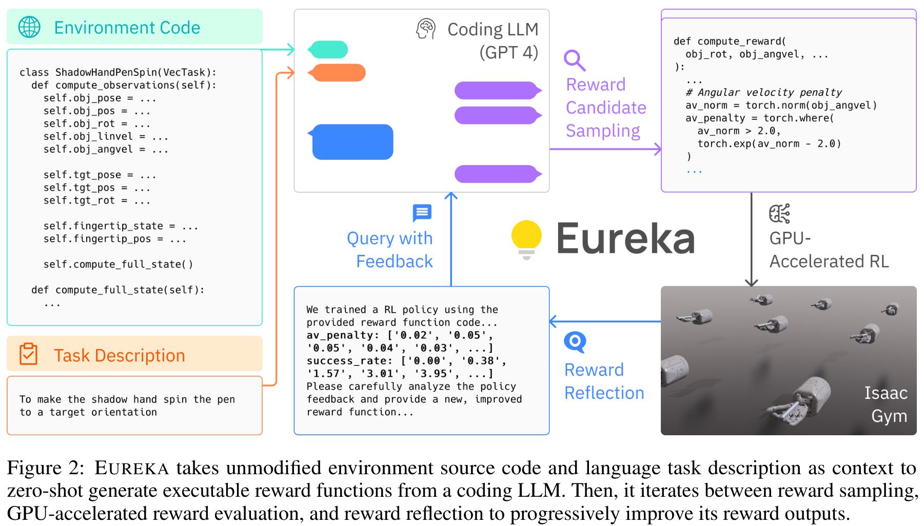
The Eureka diagram starts from environment code and a task description, generates reward code, trains and evaluates a policy with it, then uses the results to revise the reward. The authors’ project description of the components and paper, sections 2–3 clarify the division of roles.
Note three features. The inputs include the task and available environment variables. Evaluation includes actual policy training. Feedback guides the next edit to the reward code. This goes beyond asking an LLM once to write a good reward.
The paper describes reward reflection using individual reward components and policy-training statistics. These records reveal whether a term dominates, barely changes, or encourages unintended behavior. Giving that feedback in the LLM’s context differs from fine-tuning its parameters.
#Executable code alone does not establish reward quality
Evaluate a generated reward for computability, behavioral preferences, and actual learning effects.
First, can it be computed? Check input variables and units, batch dimensions, output format, and finite values. A candidate referencing a missing state variable or producing NaN fails before a performance comparison.
Second, does it prefer the intended behavior? Test simple counterexamples such as repeating in place, moving back and forth, maintaining contact, or terminating early. Passing a few counterexamples offers no guarantee across the entire action space.
Third, does it help training? Train policies under equal budgets and compare common success and failure criteria. Reserve test conditions from candidate revision.
Separate the door-opening success check from the code that generates reward candidates. If a candidate writer can edit the success check, it can change the evaluation rule instead of improving behavior. Structure the experiment so that it cannot modify that check.
#Three questions to check understanding
1. Is 0.5 points for handle contact always a good reward?No. Return depends on when, how often, and under what conditions the reward is paid. A one-time milestone and a per-step payment can define different objectives.
2. Does potential-based reward shaping resolve every failure?No. Optimal policy preservation under specified assumptions differs from efficiency, stability, and safety in finite training. Mishandling the terminal boundary can invalidate even the rank-preservation premise.
3. If the LLM produces good reward code, has the robot finished learning?No. Code proposal, policy learning, and independent evaluation are distinct. Code that looks good still needs performance validation on the actual policy.
#How the five slides fit together
Slide 16 introduces rare success rewards. Slide 17 uses door opening to identify intermediate signals. Slide 18 distinguishes true goals from proxies, and slide 19 separates optimization from evaluation. Slide 20 connects reward design and policy learning as two distinct loops.
The central question is “Does a policy trained on the reward achieve the original goal more often?” It applies whether a human or an AI designed the reward.
Next, Self-Improving AI 05 — AI That Designs Rewards and AI That Evaluates Answers covers slides 21–25, comparing reward-design research and distinguishing the training signals in RLHF and RLAIF.
#Further reading
NTU Machine Learning 2026 course information
| Source | Where to read | Connection to this article |
|---|---|---|
| Hung-yi Lee, NTU Self-Improving | PDF pages 16–20 | Main lecture sequence and notation |
| Scott Niekum, UMass CS 690 Reward Specification | PDF pages 4, 5, and 11 | Sparse and dense rewards, potential-based shaping, overfitting |
| Ng, Harada, Russell, ICML 1999 | Section 2.2 and section 3, Theorem 1, PDF pages 3–4 | Reward transformations and conditions for policy preservation |
| Booth et al., AAAI 2023 | Paper and authors’ research materials | Overfitting and task misspecification in trial-and-error reward design |
| Ma et al., Eureka project paper | PDF page 2, Figure 2, and sections 2–3 | Reward generation, policy training and evaluation, reward reflection |
| Eureka authors’ project | Components and public task examples | Distinguishing reward generation from policy learning |
Reproducing the calculations in Python
The following reproduces the three illustrative calculations without external packages.
from math import isclose


def discounted_return(rewards: list[float], gamma: float) -> float:
    """Finite-horizon discounted return for the illustrative examples."""
    if not 0.0 <= gamma <= 1.0:
        raise ValueError("gamma must be in [0, 1]")
    return sum((gamma ** t) * reward for t, reward in enumerate(rewards))


def main() -> None:
    # Independent fixed-probability trials, not an RL sample-complexity bound.
    p, trials = 0.001, 100
    chance = 1.0 - (1.0 - p) ** trials
    print(f"Success within 100 trials: {100.0 * chance:.4f}%")
    print(f"Expected trials to first success: {1.0 / p:.0f}")

    # A stays in contact; B succeeds immediately and terminates.
    contact_return = discounted_return([0.5] * 20, gamma=0.99)
    success_return = discounted_return([1.0], gamma=0.99)
    assert contact_return > success_return
    print(f"Repeated contact / immediate success: {contact_return:.6f} / {success_return:.6f}")

    gamma = 0.9
    rewards = [0.0, 0.0, 1.0]
    potentials = [-1.0, -0.6, -0.2, 0.0]
    if len(potentials) != len(rewards) + 1:
        raise ValueError("One potential is required for every visited state")
    shaped = [
        reward + gamma * potentials[t + 1] - potentials[t]
        for t, reward in enumerate(rewards)
    ]
    original_return = discounted_return(rewards, gamma)
    shaped_return = discounted_return(shaped, gamma)
    boundary_identity = (
        original_return - potentials[0]
        + gamma ** len(rewards) * potentials[-1]
    )
    assert isclose(shaped_return, boundary_identity, rel_tol=0.0, abs_tol=1e-12)
    assert isclose(shaped_return, 1.81, rel_tol=0.0, abs_tol=1e-12)
    print("Shaped rewards:", [round(value, 2) for value in shaped])
    print(f"Original / shaped return: {original_return:.2f} / {shaped_return:.2f}")


if __name__ == "__main__":
    main()
The first calculation finds the chance of a rare success under independent trials. The second checks that repeated intermediate rewards can outscore final success. The third verifies cancellation of potential terms at the boundaries. We use isclose to avoid exact equality comparisons between floating-point results as though they were identical strings.
Before applying the code in an experiment, define termination rules, time limits, and evaluation environments. An identity verified in a numerical example does not establish convergence for neural network training.