A model can generate its own learning signal. Whether its answers grow more accurate as it follows that signal is a separate question. This lesson examines the limits of self-training and the use of brief adaptation at test time.
Part 6 — Does greater confidence make an AI more accurate? examined self-evaluation, majority voting and entropy. We now look at using the input itself as a learning signal and briefly updating parameters at test time.
Video guide by slide
| Slide | Video segment | Topic |
|---|---|---|
| Slides 31–32 | 31:13–31:57 | How well self-rewarded learning works and the URLVR paper |
| Slide 32 | 31:58–32:52 | Comparing learning curves for majority-vote and ground-truth rewards |
| Slide 33 | 32:52–33:34 | Initial gains and subsequent declines across five methods |
| Slide 34 | 33:34–34:46 | Connecting inputs, learning signals, parameter updates and new outputs |
| Slides 34–35 | 34:46–36:00 | Limited adaptation and its connection to Lecture 8 from 2025 |
#Slide 31 — Can the input itself supply a learning signal?
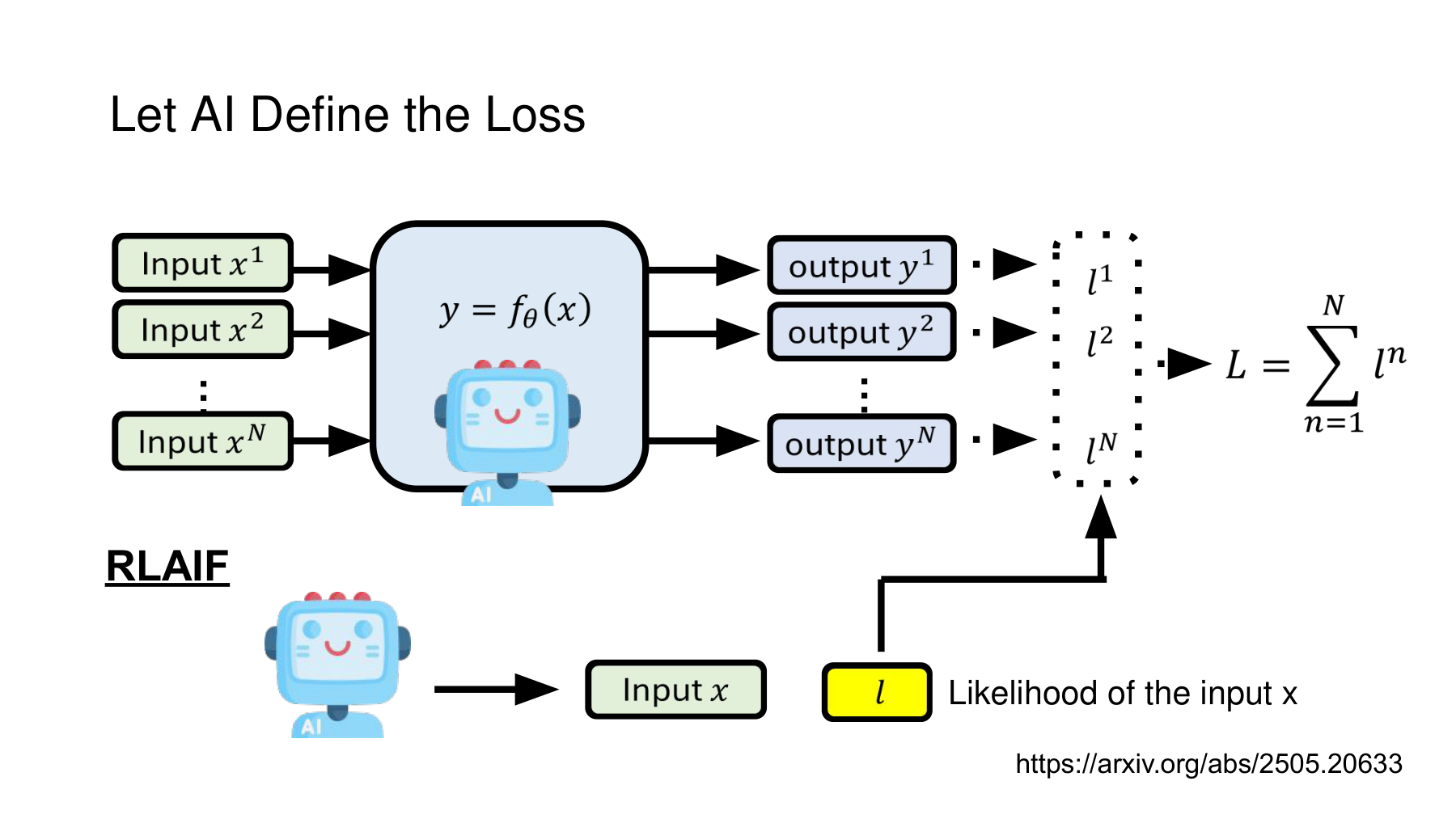
The upper half shows a familiar arrangement: the model produces outputs from inputs and aggregates losses. The lower half adds a path based on the likelihood of generating the input x and links to a paper. The learning target shifts from confidence in the answer to how well the model predicts the sentence it has just received. Original slide 31
#Input NLL and perplexity
Hu and colleagues’ Test-Time Learning for Large Language Models, linked from the slide, proposes TLM. The method combines selective sample learning and LoRA to reduce perplexity on unlabeled test inputs. Paper §4, PDF pp. 4–5 · ICML 2025 proceedings
Write the observed input as a sequence of tokens. The following mean negative log-likelihood (NLL) scores the prediction of each token from those preceding it.
A start token can supply context for the first token. The logarithm is natural. Since the exponential function is increasing, NLL and perplexity rank objective values in the same order for the same input and length normalization. However, their gradient magnitudes can differ. A single update at the same learning rate can therefore produce different results.
Minimizing the slide’s “likelihood” literally would reverse the direction. Better prediction raises likelihood and lowers NLL and perplexity. The yellow loss box is schematic. Check the sign, logarithm and normalization in the implementation.
Worked example. Suppose the probabilities assigned to two observed tokens rise from 0.5 and 0.25 to 0.8 and 0.5.
The result tells us that the model assigned higher probabilities to the two observed input tokens. It says nothing by itself about the correctness of a future answer or the truth of the input. A model can assign high likelihood to a false statement.
#Further reading A — An experiment where input and output perplexity moved together
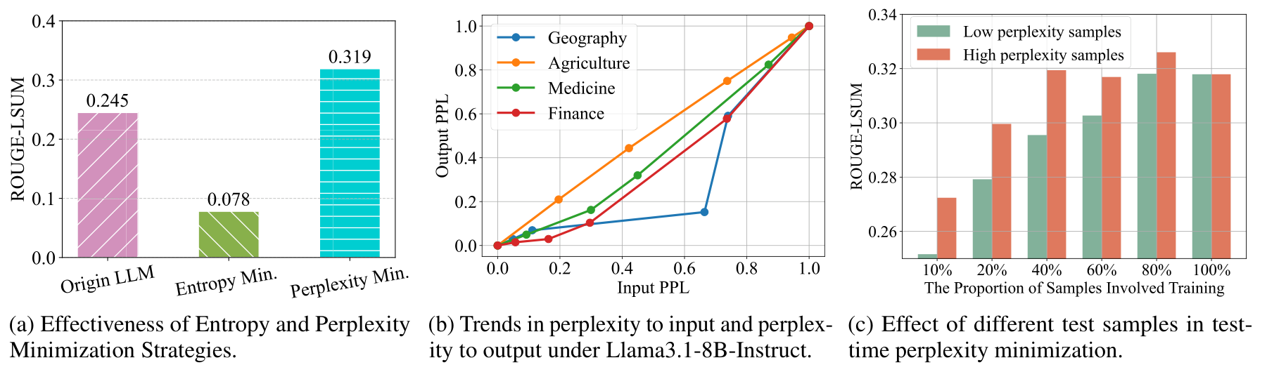
The left panel compares objectives. The middle shows normalized trends in input and output perplexity, and the right compares ways of selecting training samples. The middle axis has no universal absolute perplexity scale. The observations apply to the conditions tested. They do not establish that a better input fit always yields more correct answers. TLM Figure 1, PDF p. 4
Why does that qualification matter? The direction that reduces input loss must also improve the answer. We can inspect this condition through the gradients. For analysis, define a loss that requires access to the correct answer.
Assuming twice continuously differentiable losses in a neighborhood and a sufficiently small learning rate, a first-order Taylor expansion gives the following expression.
A positive inner product between the two gradients makes the first-order term reduce answer loss. A negative inner product reverses the effect. When it is zero, the first-order term is inconclusive. At a finite step size, the remainder also matters. The paper uses a gradient alignment assumption. The answer-loss gradient serves as an analytical tool here. An unlabeled deployment does not supply this signal. TLM equation (4), PDF p. 5
The slide’s broad use of RLAIF also needs care. TLM cannot be classified as reinforcement learning from an AI judge’s scores on that basis alone. A self-supervised update that minimizes input NLL differs from a policy-gradient update that maximizes reward. Algorithm 1 predicts a batch and then updates. The conceptual diagram on slide 34 need not use the same order. TLM Algorithm 1
#Slide 32 — Why can early gains disappear with further training?
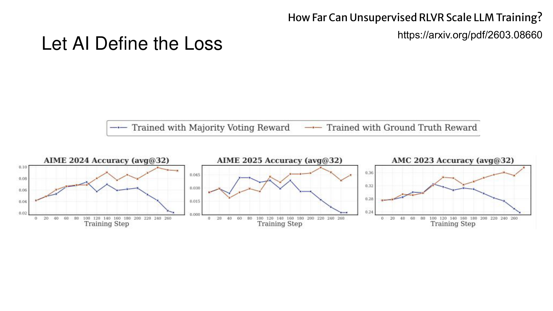
Video · 31:13–32:52. The lecturer asks how long self-rewarded learning can continue. The curves for majority-vote and ground-truth rewards initially look similar, then diverge. A “human reward” here need not mean that a person grades each training step in real time.
The accuracy panels come from Figure 2 of He and colleagues’ How Far Can Unsupervised RLVR Scale LLM Training? The experiment trains Qwen3-1.7B-Base on DAPO-17k and evaluates it on AIME 2024, AIME 2025 and AMC 2023. Paper §4.1.1, PDF p. 12
#Read the axes and the unit of evaluation
The horizontal axis gives the training step. Each panel uses a different evaluation dataset, and their vertical ranges differ. Line heights cannot be compared directly across panels. avg@32 is mean accuracy across 32 generated answers per problem. By contrast, pass@32 counts a success if any one of the 32 answers is correct. Figure 2 evaluation setup
The figure reports accuracy measured separately against ground truth. The proxy reward used during training is a different quantity. Training can omit answer labels while evaluation still requires them. “Unsupervised” describes the signal at this training stage. Pretraining data, human-defined tasks, reward rules and evaluation design still matter.
#What a majority vote verifies
Consider a simple procedure that generates K answers to one question and uses the most frequent answer as a pseudo-label.
When the pseudo-label agrees with the correct answer, both rewards can point in the same direction. When they differ, training the model to produce the pseudo-label more often can preferentially reward a wrong answer. An implementation also needs rules for extracting answers, recognizing equivalent answers and breaking ties. Counting “0.5” and “1/2” separately mistakes different notation for disagreement.
Worked example: three independent binary answers. Let p be the probability of a correct answer. Assume the answers are conditionally independent and share a single wrong alternative. The probability that a majority of three answers is correct is then as follows.
Majority voting benefits a model that already favors the correct answer and can worsen performance when it favors the wrong one. This calculation depends on its assumptions. Language models have more than two possible answers, and their samples can share a misconception or reasoning pattern. Generating several answers does not automatically provide independent verification.
Tracking whether proxy reward rose is insufficient in practice. Track proxy reward, ground-truth performance and output diversity separately. Without access to correct answers, an operating system cannot simply read off the onset of degradation as we can in this figure.
#Slide 33 — Five methods, different failure patterns
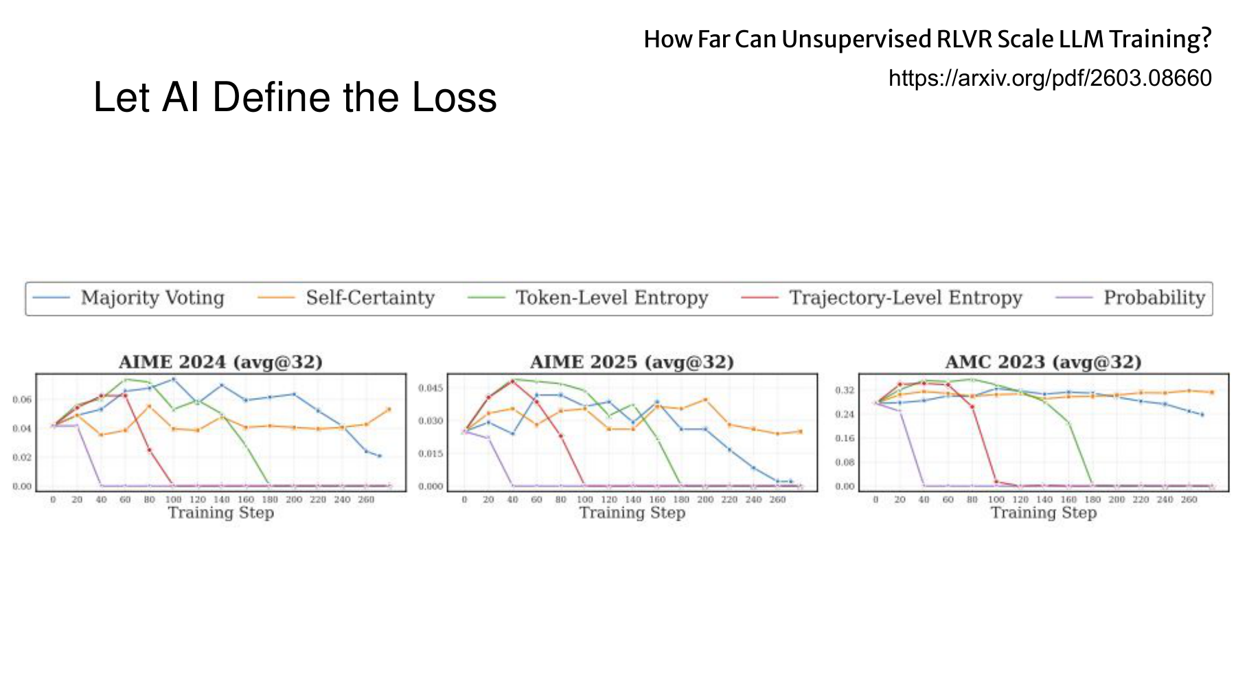
Video · 32:52–33:34. The lecturer compares the stability of five methods. Self-training can provide early gains. Problems may emerge as the model continues to follow the same signal.
The figure includes majority voting, Self-Certainty, token-level entropy, trajectory-level entropy and probability-based reward. Only some curves fall to zero during the displayed training window. This figure cannot establish inevitable collapse for every model, reward and form of self-training. Paper Figure 3 and §4.1.2, PDF p. 13
The paper analyzes several patterns in this setting: gradual decline, excessively short answers and repetition. Implementation details and length handling matter. A weakness of one probability reward does not establish an inherent defect in all probability-based methods. Failure analysis
#How does a score influence the form of an answer?
Suppose we score a complete answer using the product of conditional token probabilities. The probability of a finite token sequence, including termination, factors as follows.
To isolate the length effect, consider a hypothetical example in which every conditional probability is 0.9.
The score does not directly measure completeness. A shorter sequence can win by omitting a necessary explanation. Mean log probability can adjust for length without guaranteeing correctness. Conversely, minimizing average token entropy can favor easy-to-predict repetitions. Try constructing a counterexample that exposes what the proposed score misses.
To detect reward hacking, monitor answer length, repetition, the fraction of valid answers, termination and refusals alongside accuracy. An arbitrary length limit does not correct a mismatch between the reward and the objective.
#Further reading B — Small datasets and small batches
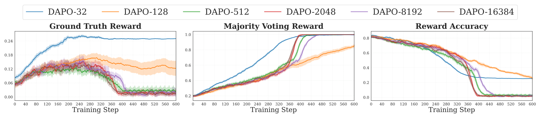
Figure 6 varies total dataset size while holding batch size at 32 and optimization steps at 600. Performance remained stable over the observed interval with 32 and 128 samples and declined in larger settings. The value 128 is not a general safety threshold for other models. Paper §5.1, PDF p. 16
Here 32 and 128 refer to the total number of distinct training problems, not merely the minibatch size. Holding the number of steps fixed changes the frequency with which each problem is encountered. Dataset size changes the training experience as well as the count of examples.
Additional calculation. With 32 inputs in each batch and 600 updates, the input count is 19,200, excluding generated rollouts. Assuming uniform use, each problem appears 600 times on average with 32 problems, 150 times with 128 and 37.5 times with 512.
These are equivalent input exposures, excluding rollout generations. Record dataset size, batch size, steps, generation count and actual parameter displacement separately. Keeping small-data findings distinct from large-scale training results helps explain the following TTT setup.
#Slide 34 — Briefly updating parameters during inference
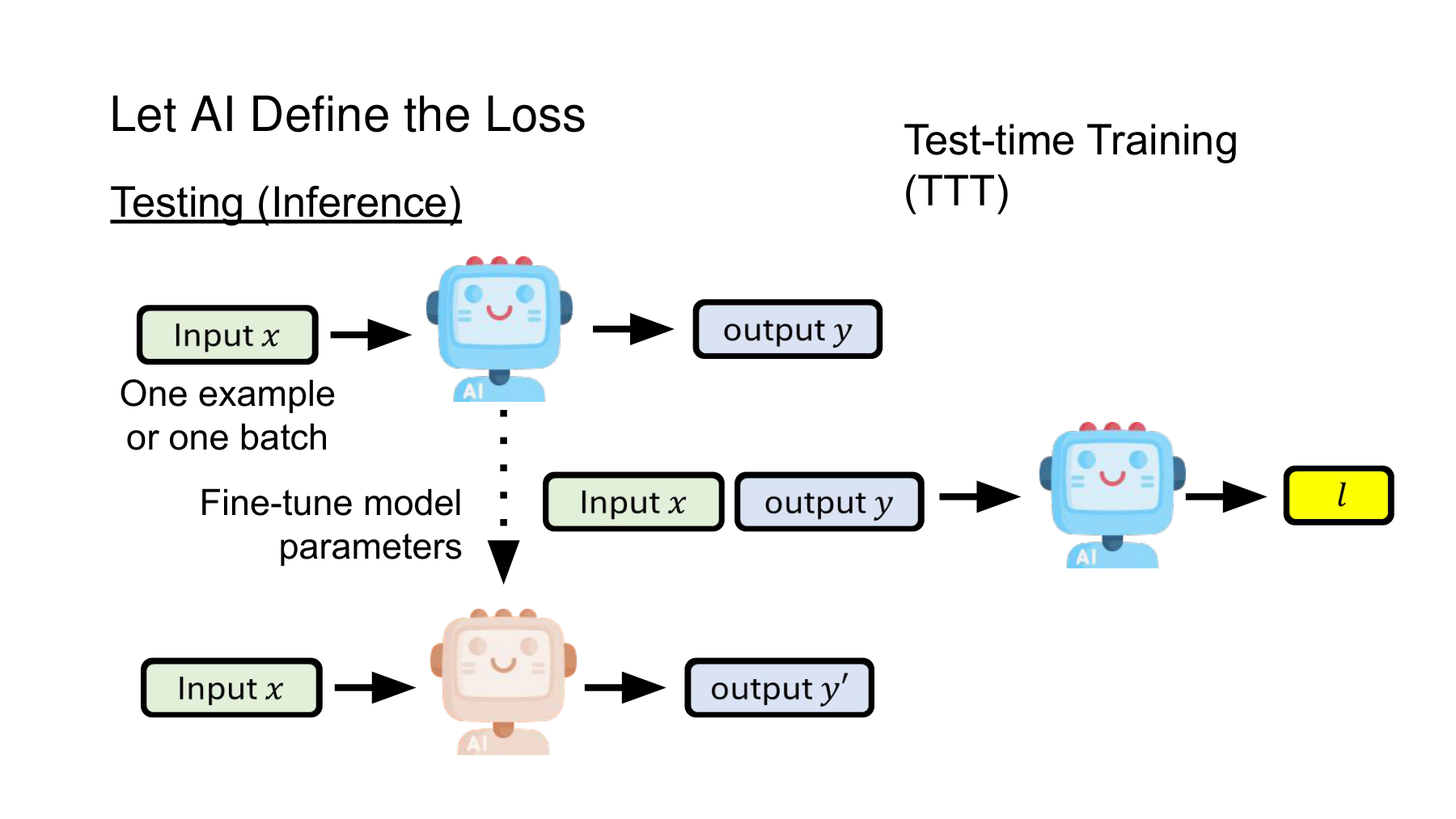
Video · 33:34–34:46. The lecturer traces a path from a test input to an output, a parameter update using a self-generated signal, and a new output for the same input. The user sees the final answer. A training step takes place inside the procedure.
#Distinguishing the input from its answer label
In ordinary fixed-model inference, the model produces an output without changing its weights. In the test-time training (TTT) considered here, unlabeled test inputs update the parameters designated as trainable. The update receives no answer labels. Sun and colleagues’ 2020 TTT method illustrates this approach by converting a single test input into a self-supervised task. Original TTT paper, §2
Here is an illustrative general expression for gradient-based adaptation. Write for the trainable parameters and for a test input or batch. Other weights may remain fixed.
The choice of trainable parameters, loss and number of updates determines the method. Check precisely which adapters, normalization coefficients or feature extractors are updated before drawing conclusions about the full network.
TTT need not begin by generating a complete answer y. Input-token NLL and auxiliary tasks such as rotation prediction produce learning signals without such an answer. Conversely, learning from rewards on sampled answers requires a procedure such as policy gradient. One cannot simply differentiate through discrete tokens. The general expression assumes a suitable objective has already been constructed.
#Further reading C — Thinking longer and training at test time
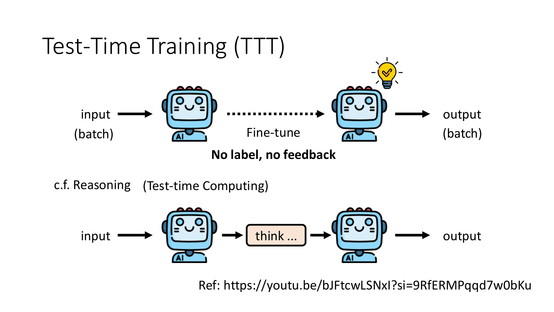
The upper half of the 2025 slide shows parameter fine-tuning, and the lower half increases inference computation. Generating a longer reasoning trace or selecting from more candidates differs from updating weights with a loss. NTU GenAI-ML 2025, Post PDF p. 86
| Method | What changes | Question to ask |
|---|---|---|
| Longer reasoning or candidate generation | Generated tokens and candidate pool | Did computation increase with fixed weights? |
| In-context examples or retrieved material | Input context read by the model | Did the model receive additional information? |
| Gradient-based TTT | Designated trainable parameters | Was there a loss, backward pass and update? |
These distinctions can coexist in one system. For example, the model can generate candidates, select a pseudo-label and then train on it. Record candidate selection and parameter learning separately. Similarly, storing more intermediate computations in a KV cache provides no evidence by itself of weight learning.
#A small step can still go in the wrong direction
A small amount of learning offers no guarantee. Reduce the gradient alignment argument to one variable and calculate the update direction using simple quadratic losses.
The proxy loss falls while the true target loss rises. Brief adaptation can limit the extent of failure, but it leaves a misaligned objective misaligned. Assess the real goal independently as well as recording update counts.
#Slide 35 — After adapting to one problem, which state should persist?
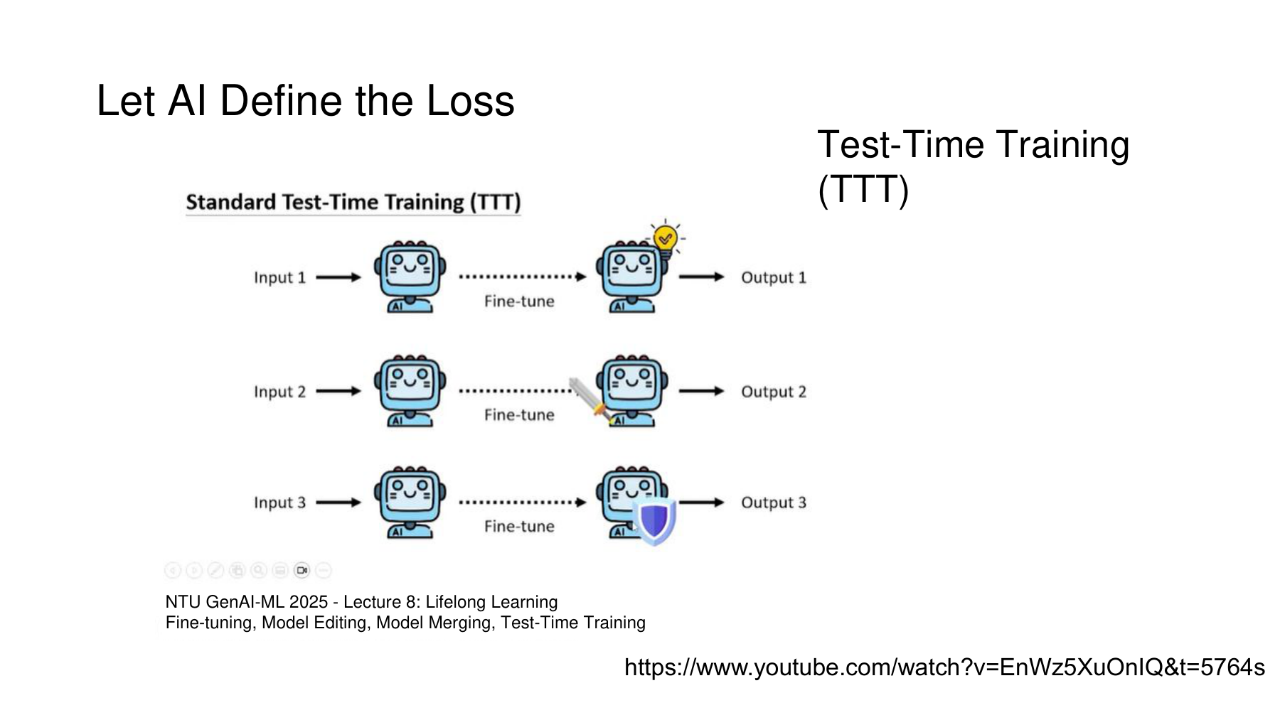
Video · 34:46–36:00. The lecturer connects small datasets and limited updates to TTT and refers readers to Lecture 8 from 2025 for further detail. A small adaptation budget alone cannot establish safety across deployment settings.
The slide links to 1:36:04 in Lecture 8, 2025. The three rows on slide 35 illustrate standard TTT restarting from the base model for each input. Post PDF p. 95
#Episodic and continual adaptation
Write U for the update on one input. The following notation compares resetting the model between inputs with carrying updates forward.
Episodic adaptation discards weight changes before processing the next input. Continual or online adaptation inherits previous updates. This can help the model track a changing distribution and can also propagate a bad update to later inputs. The original 2020 TTT paper specifies this initialization difference for its standard and online variants. Sun et al., §2, PDF p. 2
Worked example. Use the following simplified auxiliary loss for each input. Here a denotes a hypothetical target for the auxiliary task.
| Procedure | Result after first update | Starting value for second input | Result after second update |
|---|---|---|---|
| Reset for each input | 1 | 0 | −1 |
| Carry the previous value forward | 1 | 1 | −0.5 |
The same inputs and learning rate produce different second results. Reversing the order in the continual setting gives a final value of +0.5. Record input order and reset rules when comparing results. An implementation should also specify what happens to optimizer momentum, statistics and adapter state when weights are reset.
#Further reading D — Constructing a loss without the target label
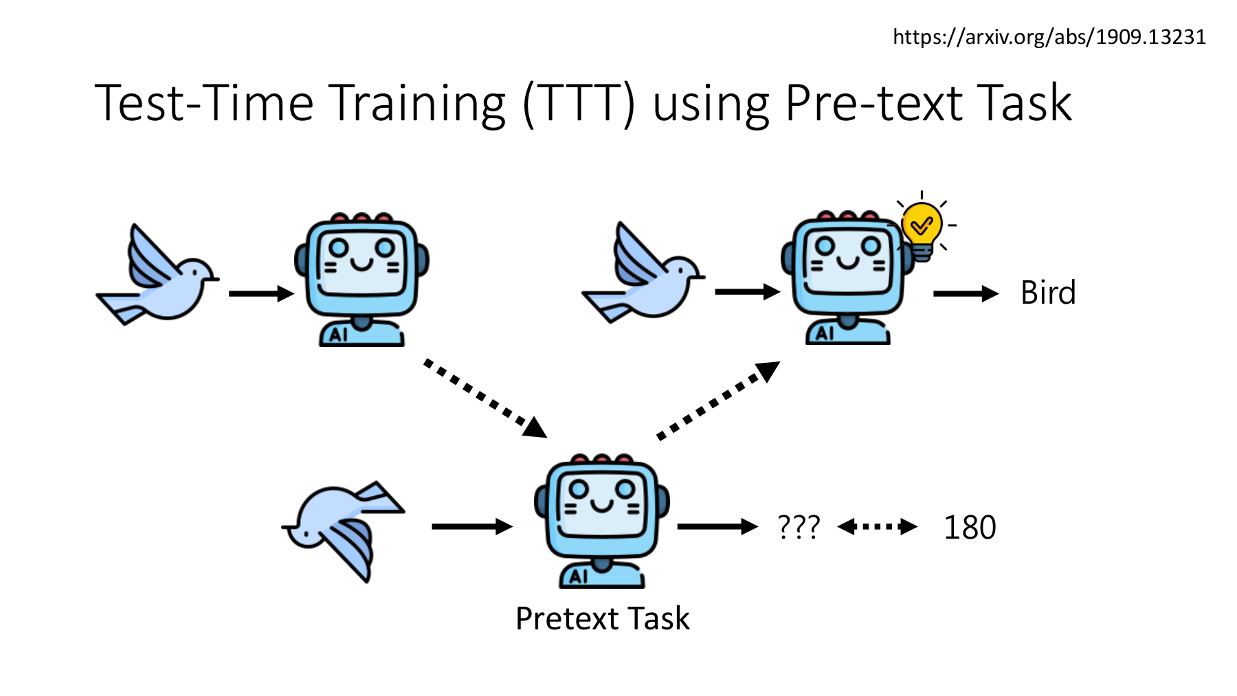
The main task identifies a bird species. The auxiliary task predicts how far the image has been rotated. The species label may be unavailable, but the program knows it rotated the image by 180 degrees. The transformation itself supplies the pretext-task label. Self-supervised learning need not copy the model’s own answer as a target. NTU Post PDF p. 94
The original TTT paper shares a feature extractor between rotation prediction and the main task. At test time it adjusts the shared part using the auxiliary loss and then predicts the main task. Check independently whether this relationship transfers to another task. Sun et al., §2, equations (2)–(3)
For example, an orientation-sensitive task can need a different representation from one that should ignore changes in orientation. Easy-to-generate labels alone do not make a good auxiliary task. Identify which information or invariance the task teaches and whether it helps the final prediction.
#What to specify before an adaptation experiment
Set the following conditions before running the experiment.
| Item | Specify in advance |
|---|---|
| Accessible data | Test inputs only, or additional sources, tools or human feedback |
| Parameters to update | Which layers, adapters or normalization coefficients change and which stay fixed |
| Adaptation budget | Learning rate, maximum updates, batch size, generated candidates and latency |
| State lifetime | Reset per input, carry state forward, and conditions for rollback |
| Evaluation | Performance relative to a fixed model, failure and repetition, regressions on other tasks, computational cost |
Adapting on test inputs can be part of a TTT evaluation protocol. Concealing that access and reporting the comparison as fixed-model inference distorts the result. Also distinguish using test answers to construct a loss from repeatedly inspecting test scores to select the learning rate or stopping point. Document the roles of validation and final evaluation data separately.
In machine vision, one can test adaptation to lighting or noise changes. In real-time robot control, latency and recovery after failure also matter. Assess input changes, estimation performance and timing separately, and retain a base model to restore if adaptation fails.
#How the five slides fit together
Slide 31 explains how the input can supply a learning signal. Slides 32–33 distinguish early gains from long-term self-reinforcement. Slides 34–35 specify what to update and reset when applying the idea to a limited set of test inputs.
Evaluate self-training by the source of its signal, its connection to the goal, the scope of updates and independent evidence. Falling proxy loss, rising accuracy and sustained generalization measure different things.
Check 1. Does lower input perplexity imply a correct answer? It shows better prediction of the input tokens. A link to answer correctness needs conditions and evidence.
Check 2. Does the 128-sample condition in Figure 6 set a safety limit for all models? It is an observation for a particular model, dataset, reward and budget. Keep total dataset size distinct from minibatch size.
Check 3. Does generating more inference tokens count as TTT? That alone is insufficient. The gradient-based TTT in this article includes a parameter update.
Next is Part 8, original slides 36–40. The lecture’s “Math Warning” section examines how to compute and optimize entropy in an enormous output space. Continue to Self-Improving AI 08 — Finding the missing gradient in entropy minimization.
#Videos, slides and papers
| Resource | Location | Connection |
|---|---|---|
| NTU Self-Improving lecture, first half | 31:13–36:00 | Self-rewarded learning and test-time adaptation |
| NTU Self-Improving PDF | May 8, 2026 lecture, pp. 31–35 | Self-rewarded learning and test-time adaptation |
| Test-Time Learning for Large Language Models | arXiv v1, May 27, 2025, Figure 1, Algorithm 1, §4.1 | Input perplexity and conditional gradient alignment |
| How Far Can Unsupervised RLVR Scale LLM Training? | arXiv v1, March 9, 2026, Figures 2, 3 and 6, §§4.1 and 5.1 | Early improvement, later decline and dataset-size comparisons |
| NTU GenAI-ML 2025 Lecture 8, Post | Fall 2025, PDF pp. 86 and 94–96 | TTT, inference compute, rotation as an auxiliary task, reset and accumulation |
| Original TTT paper | ICML 2020, §§2 and 4 | Self-supervised TTT procedure and conditions of use |