A factory adds a second exposure to its camera inspection routine. It catches defects that used to disappear in blurry images. But now even a sharp image can time out while the system waits for another exposure. The camera and the vision model are unchanged. Can changing the order of operations cost the system a skill it had yesterday?
Chapter 19 showed how to check an earlier capability after adapting a model to a new input. Here the change happens in the harness, the code, prompts and tool calls around the model. Pages 31–32 of the second lecture measure how much of an earlier capability survives. Pages 33–35 ask whether the improver that edits the harness has also changed. The camera is a worked example. The papers evaluate customer-service workflows and coding agents.
Worked examples Lost cases · Success rate · Retention ratio · Proposal and acceptance · Inspection mix · Fixed editor
Video guide by slide
| Part II page | Lecture video | What to listen for |
|---|---|---|
| 31 | 30:18 | Can changing only the harness erode an old capability? |
| 32 | 31:01 | What else should we measure as workflow code gets longer? |
| 33 | 33:12 | How do we distinguish the changing agent from its update rule? |
| 34 | 33:51 | How do the existing code and execution results inform a proposed edit? |
| 35 | 34:35 | What changes when the editor is held fixed? |
Each time link goes to the spoken discussion of that topic. NTU course materials for May 22, 2026
#Part II, page 31 — A harness can forget while model weights stay fixed
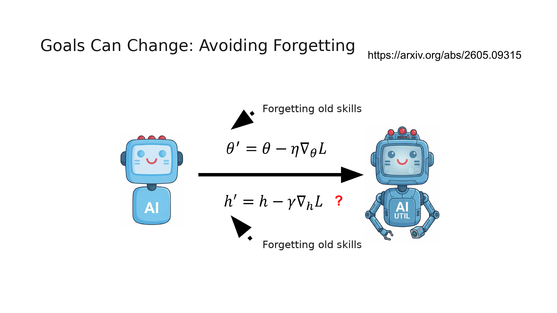
An inspection camera sees the same image and assigns it the same defect probability, yet a scratch it detected yesterday goes unreported today. What changed? Imagine adding a rule to reduce false alarms from reflections: issue an alert only after two consecutive frames show a defect. A fine scratch visible for just one frame can still clear the classifier threshold and then disappear at the alert stage. In this example the change lives in the harness that converts predictions into alerts.
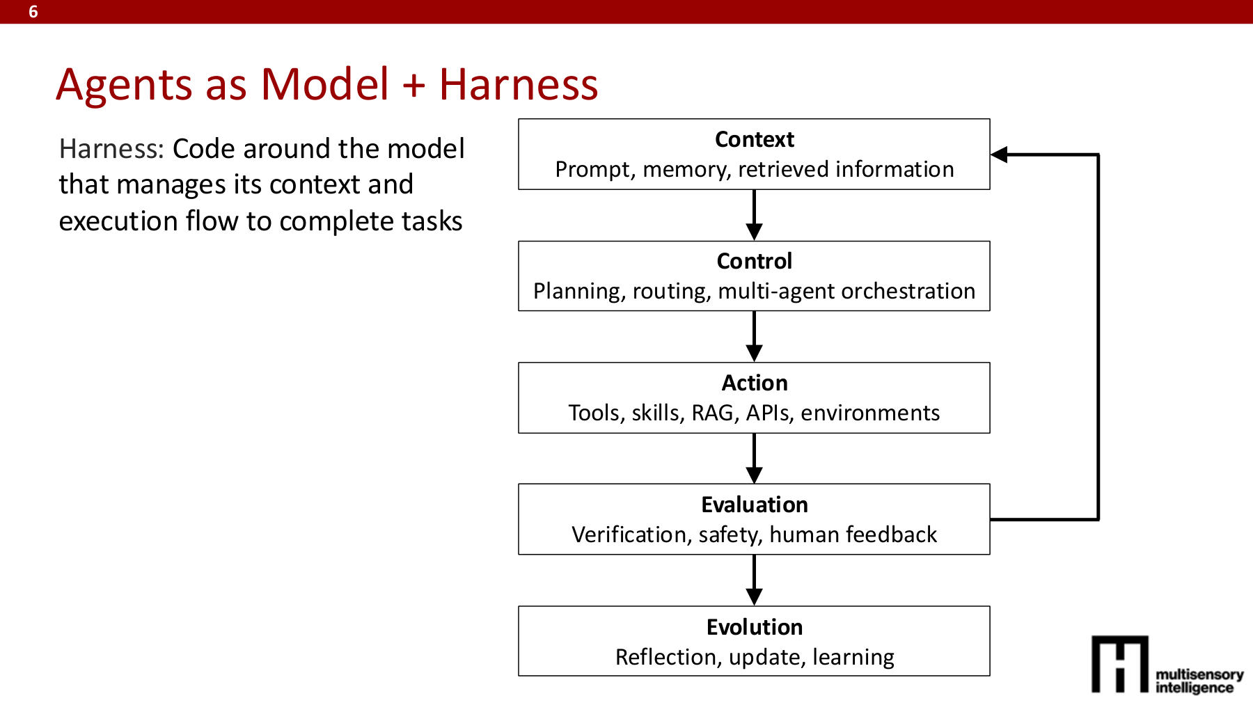
Page 6 of MIT’s harness lecture breaks down the jobs of the code around a model into context, control, action, evaluation, and evolution. For the inspection camera, the previous frame’s score supplies context, the two-frame branch supplies control, and sending an alert is an action. Matching alerts to labeled clips to find missed scratches is evaluation. Revising the rule in light of those results is evolution. A change in control flow can alter both alerts and measured performance even when the defect scores stay the same. MIT, Harness Evolution, p. 6
The upper equation on the slide moves model weights θ in the negative gradient direction, with learning rate η setting the step size. The lower equation puts the harness h in the same position and adds a red question mark. Source-code edits such as adding a validation step or reordering tool calls have no ordinary derivative with respect to the code itself. We can still run a candidate harness and measure what changed on old and new tasks. Yu and colleagues call the part of the system being updated its capability state R. In their experiments R may be a workflow, a skill and tool collection, model weights, or memory. NTU slide 31 · Yu et al., §§2 and 3.3
#Worked example 1. How many cases were lost if the net drop was five?
Run both versions on the same 100 labeled inspection clips. Suppose both versions classify 72 correctly, only the original gets 8 right, only the revised version gets 3 right, and both miss the remaining 17. These are illustrative counts for a camera that encounters both reflections and fleeting scratches.
The success rate fell five percentage points, but the revision lost eight previously correct cases. Its three newly correct results offset part of that loss in the aggregate. Of the 80 cases originally classified correctly, 72/80 = 90% remained correct. Dividing the final score by the initial score gives 75/80 = 93.75%, which includes the three gains as well. Pairing the same clips across versions lets us distinguish the two quantities.
#Part II, page 32 — Read the denominators behind code growth, success, and retention
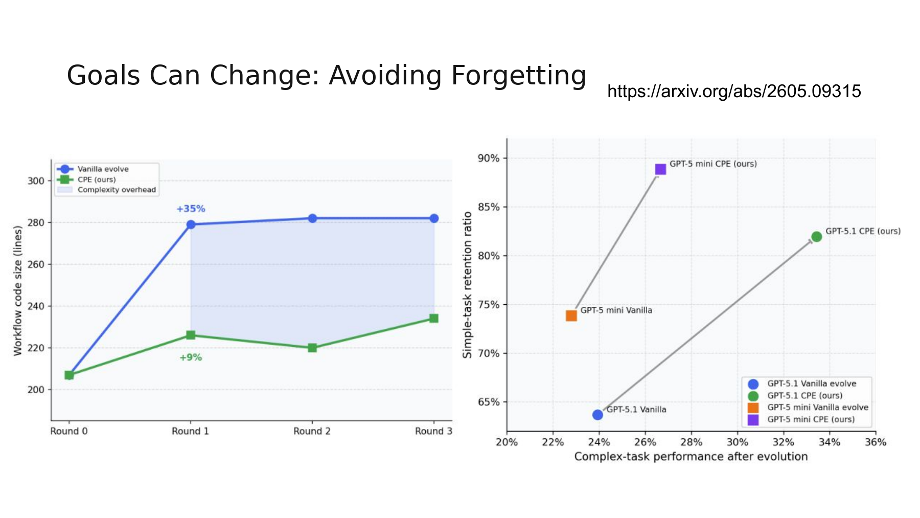
Yu and colleagues started with the same simple-task workflow for each of three τ²-Bench domains: airline, retail, and telecom. Two branches received failed complex-task trajectories and the same budget to revise the workflow. Vanilla evolution lets the optimizer rewrite the workflow from those failures. Capability-Preserving Evolution (CPE) also gives the editor anchors from the seed workflow, including task objectives, output constraints, and behaviors that prevent failures. The authors used the first 20% of complex tasks for evolution and reserved the remaining 80% for evaluation. They retested the entire simple-task set to measure retained performance. Yu et al., Fig. 2 and Table 1 · Appendix C.2 and Table 9
The left panel counts lines of workflow code during evolution on complex airline tasks. From the starting point to the first revision, code length grew by about 35% under vanilla evolution and 9% under CPE. Both annotations refer to that first round. Figure 2(a) in the paper shows how extra validation can change behavior. A check that catches malformed intermediate outputs on a complex request can reject an unusual but valid action on a simple one, cutting short an episode the agent could have recovered. Code length alone cannot reveal which behavior was lost. The right panel measures the consequences. NTU slide 32 · Yu et al., Fig. 2(a–c)
#Worked example 2. Where does the 52.8% simple-task success rate come from?
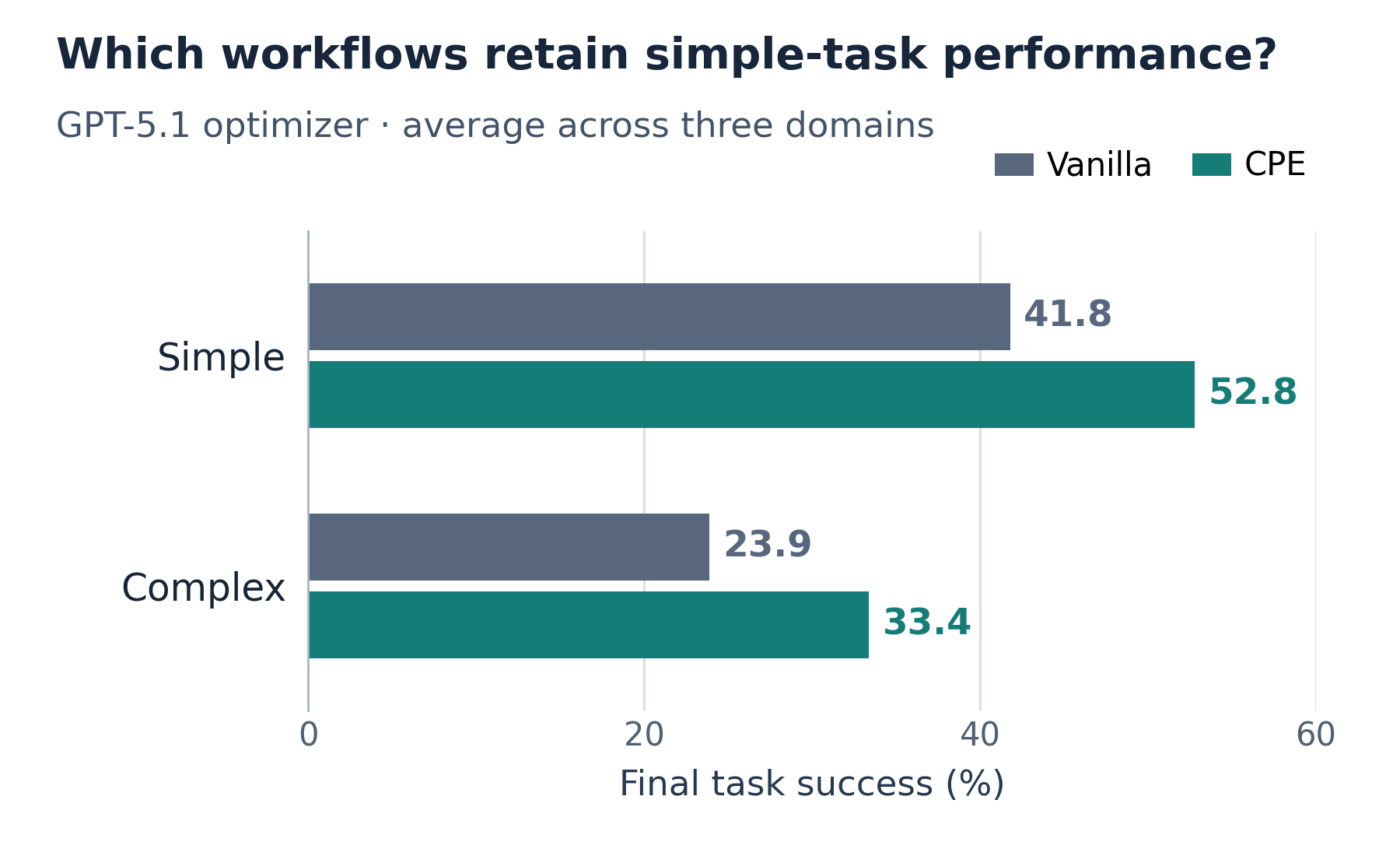
Read the GPT-5.1 simple-task scores in Table 1 in airline, retail, and telecom order. A macro average gives each domain one vote. The calculation below uses the percentages printed for each domain.
Compare the two final versions that started from the same seed. CPE scores 52.8 − 41.8 = 11.0 percentage points higher on simple tasks and 33.4 − 23.9 = 9.5 points higher on complex tasks. Retail accounts for most of the complex-task difference (20.3% to 45.3%). The two airline scores are both 37.5%. The domains have different numbers of tasks, so pooling all solved cases over all tasks would give a different average. Yu et al., Table 1 · Task counts by domain, Table 5
#Worked example 3. Why does the same CPE workflow reach about 82% in the right panel?
The horizontal axis is final complex-task success. The vertical axis measures how much of each domain’s initial simple-task performance remains. The initial GPT-5.1 values in Appendix Fig. 7(a) are 71.4% for airline, 76.7% for retail, and 45.8% for telecom. Divide each final score by its own domain’s initial score, then average the ratios to reproduce the heights in Fig. 2(c). The calculations use the rounded values printed in the paper.
The GPT-5.1 point therefore moves from about (23.9%, 64%) to (33.4%, 82%). CPE still loses some of the seed workflow’s simple-task performance, but retains more of it after adapting to the same complex-task distribution. These ratios use aggregate scores. Recovering the exact number of previously correct cases that stayed correct would require paired task outcomes. The other optimizer is labeled “mini” in Fig. 2(c) and “nano” in Table 1 and Appendix Fig. 7, so this reconstruction uses the consistently labeled GPT-5.1 series. Yu et al., Fig. 2(c) · Initial and final scores, Appendix Fig. 7(a)
#Part II, page 33 — Why is there one wrench beneath several generations of robots?
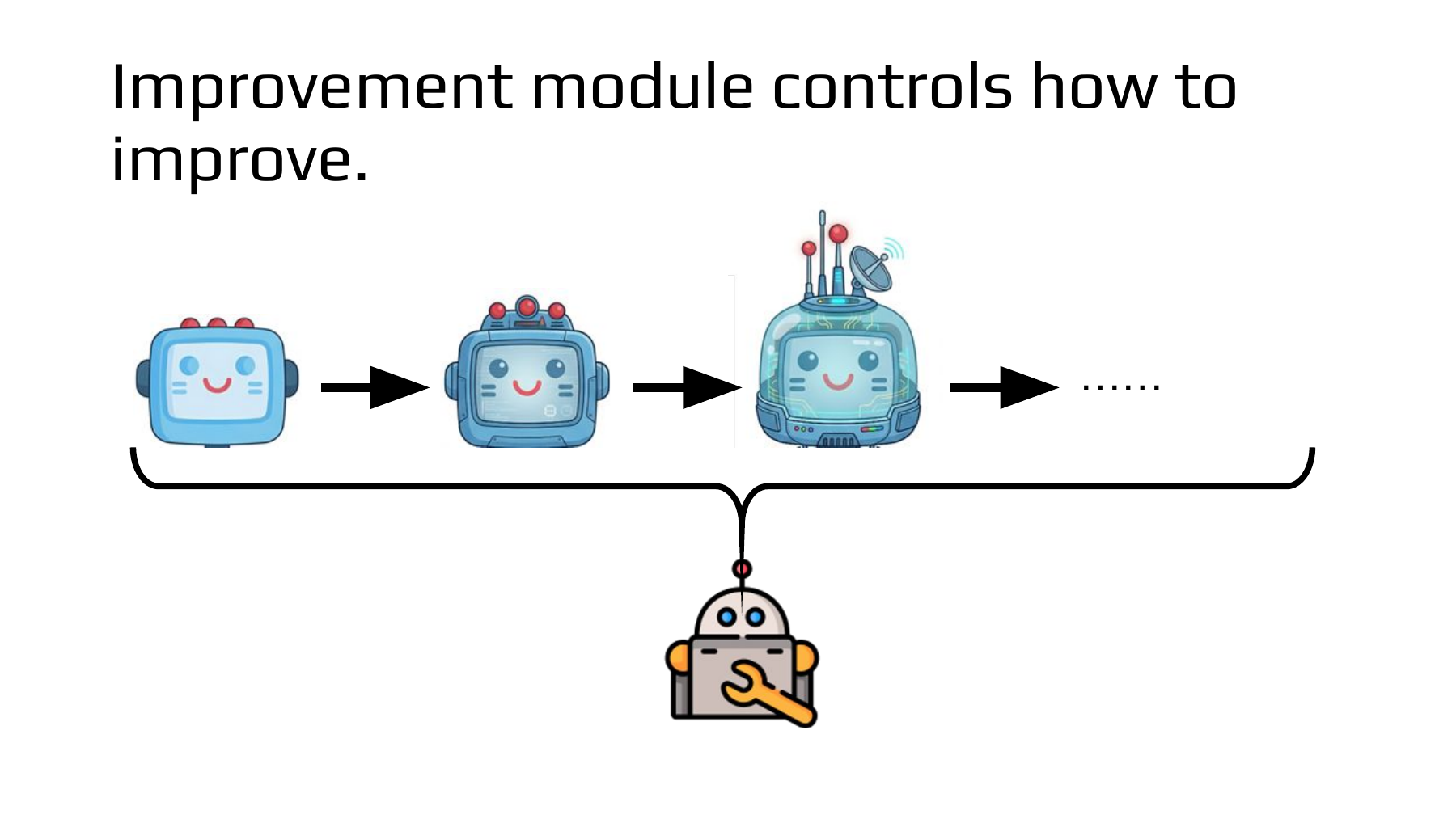
The robots’ heads and equipment change from left to right. Under the entire sequence, a single robot with a wrench sits beneath a brace. The top row shows versions of the agent that performs the task. The bottom shows the procedure that makes the next version. The same distinction applies to a camera inspection system. One procedure specifies how to inspect a part. Another uses the record of a failed inspection to revise that procedure. NTU lecture, 33:12
#Worked example 4. How many edits survive when the improvement rule stays fixed?
Let hₜ be the current harness, rₜ the trace from running the inspection, and U the rule that proposes an edit. In this hypothetical experiment, U receives the same instruction every time: read the trace and change one part of the procedure. Let S count how many of 20 validation images the candidate classifies correctly. Adopt a candidate only if its score exceeds that of the current version.
The indicator adds 1 for a correct prediction and 0 otherwise. The initial version gets 13 images right. The first proposal checks a second exposure only on dark frames. It gets 15 right and is adopted. The second proposal requires another exposure on every frame. It gets 14 right. Its comparison point is the 15 correct predictions from the current version.
| Stage | Current version correct | Candidate correct | Score carried into the next stage |
|---|---|---|---|
| First edit | 13 | 15 | 15 |
| Second edit | 15 | 14 | 15 |
The first edit raised validation accuracy by 10 percentage points. The second candidate scored 5 points below the current version, so it stays in the records. We have two edits proposed, one adopted, and zero changes to the improvement rule. Because the same 20 images informed both choices, we need images held out of selection to check whether the final harness also improves on a new camera. This adoption rule belongs to the example. The DGM discussed below keeps an archive with multiple branches.
#Supplementary paper · How a design record grows while the designer stays fixed
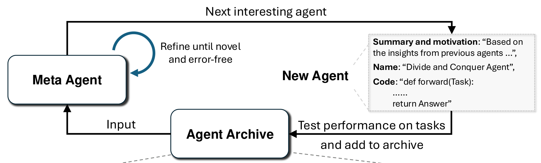
Read the Meta Agent Search diagram from Hu and colleagues from left to right. A designer, the meta-agent, reads an archive of previous designs and their validation scores, then proposes code for a new agent. Evaluation sends the new design and its score back to the archive. The next proposal thus draws on more evidence. The outer design procedure can stay the same while it produces different candidates. In the camera example, even the score and failure trace from the attempt to retake every frame could inform the next proposal. Hu et al., ADAS, Figure 1
#Part II, page 34 — Can two harnesses have the same loss and need different fixes?
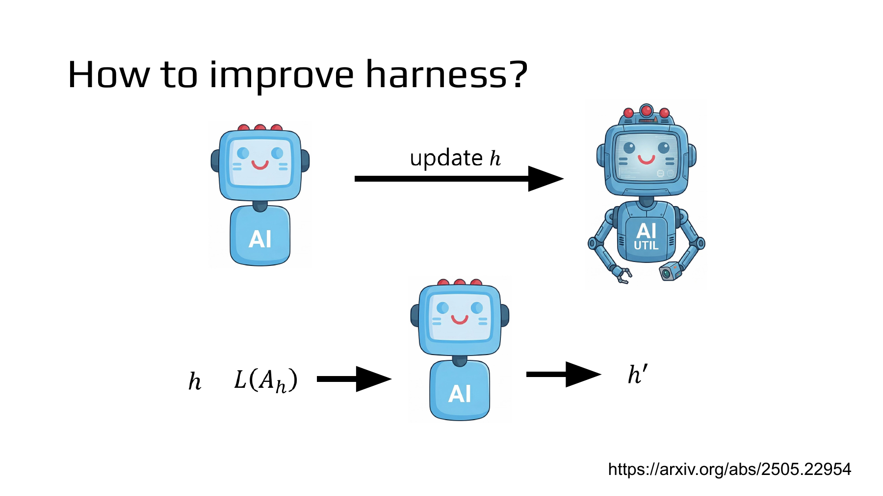
In the top row, changing the harness h gives the robot additional tools. The bottom row expands that single edit. The current harness h and the loss L(Aₕ) of the agent using it enter from the left. A proposed revision h′ emerges on the right. Lee explains that the editor can also inspect what happened when the code ran on a benchmark. A loss can summarize how often an inspection failed. A trace shows at which step it failed. NTU lecture, 34:08
Suppose each of two harnesses fails on 3 of 20 photos, a failure rate of 15%. One trace records three timeouts while waiting for another exposure. The other records three outputs missing a part number. In the first case, inspect the condition that triggers a retake. In the second, inspect the required output fields. Nothing in the number 0.15 identifies which edit to try.
#Worked example 5. When does an extra inspection pay off?
Test simple and complex frames separately on a hypothetical inspection line. On 100 simple frames, the original procedure A gets 90 right and procedure B, which adds a second inspection, gets 84 right. On 100 complex frames, A gets 40 right and B gets 58 right. Let w be the fraction of incoming frames that will be complex. Assume an error in either group has the same cost. Weight each group’s success rate by how often it occurs to obtain the expected success rate.
Subtract A’s score from B’s. B loses 6 percentage points on simple frames and gains 18 on complex ones. The two procedures therefore have a break-even point.
If 10% of the frames are complex, A scores 85% and B scores 81.4%. At 50%, A scores 65% and B scores 71%. B wins on a validation set with equal numbers of simple and complex frames. Deploying it unchanged on a line where complex frames are rare could reduce accuracy. To interpret a harness’s loss, we need to know the mix of tasks on which it was measured.
#Supplementary lecture · Using execution time to score a candidate
In his MIT lecture on AlphaEvolve, Paul Liang describes a human specifying the task and its criterion. One example is an evaluator that runs a candidate program and measures its execution time. Keeping the prompt, proposed code, and score lets the next proposal draw on prior trials. In the camera example, keeping the frames that timed out alongside the 15% failure rate gives the editor a reason to revisit the retake step. In both cases, evidence from running a candidate informs the next proposal. MIT lecture, slide 55 · Runtime and the trial record, 1:08:16
#Part II, page 35 — Which agent performs the inspection, and which one edits it?
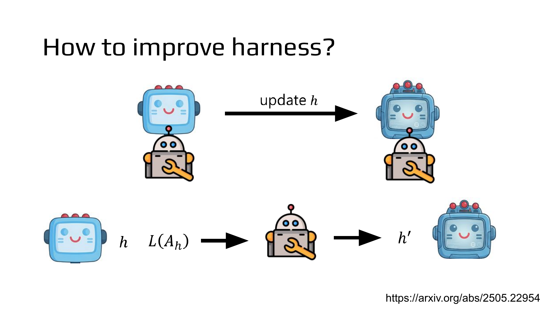
In the lower row, a robot with an orange wrench now takes the place of the agent that produced the revision on page 34. The blue robot on the left is the target of the edit. The robot with the wrench is the editor. In the top row, the same wrench icon appears beneath both the original blue robot and its successor. If the blue robot performs the task better, what would tell us whether the editor also learned to make better changes? One way to investigate is to run a comparison that keeps the editor at its initial version. NTU lecture, 34:35
In the Darwin Gödel Machine (DGM) of Zhang and colleagues, the foundation model’s weights stay fixed while the agent’s code changes. A selected agent edits its own codebase. A code-editing tool improved in this round can therefore help with subsequent revisions. The researchers specified the parent-selection procedure and evaluation system. In the paper’s fixed-editor comparison, the system keeps producing candidates while the agent used to edit them remains the initial version. DGM, §§3–4.3
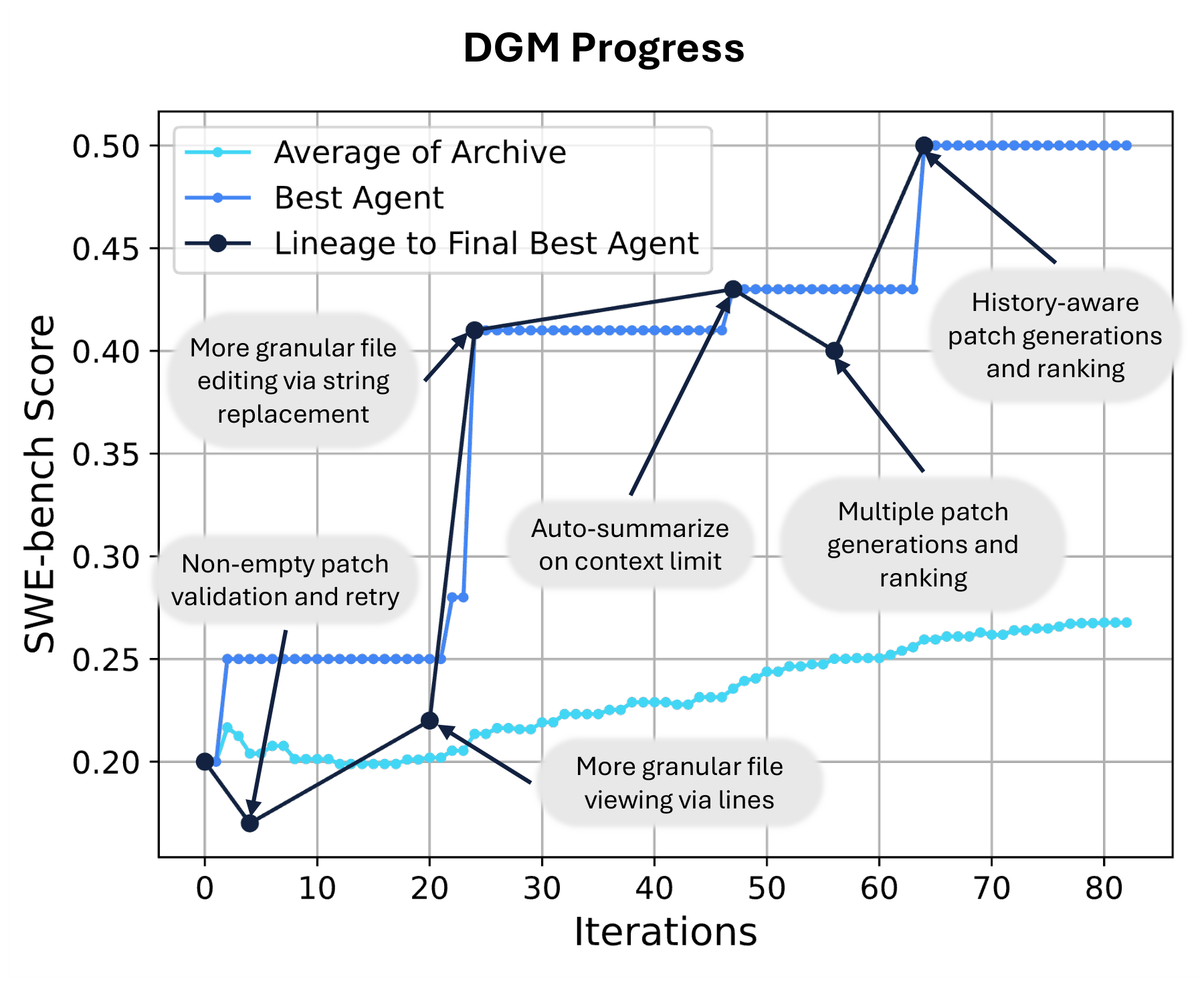
There are three lines in the right panel of Figure 3. The blue line is the highest score found anywhere in the archive up to each iteration. The light blue line averages the scores of agents with basic code-editing functionality. The dark line follows one lineage, traced backward from the best final agent through its ancestors, with two dips along the way. The average can fall while the archive record holds steady. A lower-scoring ancestor on the final lineage shows that a temporary setback can precede a useful change. It does not establish the value of every low-scoring candidate. DGM, Figure 3
#Worked example 6. What changes when the editor stays fixed?
The two rows below come from the paper’s SWE-bench experiment. The first counts problems in the evaluated SWE-bench subset. The second counts agents generated during the experiment. Identify the denominator before subtracting the two conditions within a row. DGM, appendix Table 1 · Appendix Table 2
| What was counted? | Editor fixed at its initial version | Full DGM |
|---|---|---|
| Problems solved in the evaluated SWE-bench subset | 39.0% | 50.0% |
| Generated agents retaining basic code-editing functionality | 32.5% | 51.3% |
The full DGM scored higher on both measures. The first difference concerns solving assigned problems. The second concerns the share of candidates with the basic editing capability needed for further changes. The denominators differ, so adding 18.8 points to 11.0 points would have no useful interpretation. A test of basic code editing also tells us little on its own about the chance of producing a beneficial edit. The measurements apply to this benchmark and experimental budget.
Return to the inspection line. To learn whether the new harness retained its behavior on simple frames, run it on the same old frames. To investigate whether the editing procedure improved, compare the candidates the different editors produce with the same starting version and budget. Page 36 takes that question a step further. Who can change the wrench itself, and how? Next original slide, p. 36
Figures adapted from Yu, Hu and Zhang are credited in their captions. Figure license