Training an inspection camera brings its error count from ten to zero on the same 20 held-out photos of a new part. That shows this classifier improved on these photos. Would a fresh camera adapt from fewer examples if it used the same learning procedure? To answer the second question, reset the task-specific weights and try the procedure on another task.
Chapter 22 compared rules for changing model weights. Part II, pages 46–50, begins with SEAL, which evaluates training material proposed by the model itself. We then separate an inner update that teaches a model from an outer update that revises the learning procedure using the outcomes. The cameras and calibration targets are illustrative. For the SEAL and MAML results, the paper tables specify exactly what each percentage counts.
Worked examples Rewarding edits · ARC success rate · Learning speed · Transferring a rule · Differentiating a step size · Learning an initialization · Counting shots
Video guide by slide
| Part II page | Lecture video | Question to listen for |
|---|---|---|
| 46 | 40:22 | Which self-edits should the model learn to generate again? |
| 47 | 42:02 | How does learning a task differ from improving the learning rule? |
| 48 | 44:14 | Why compare a lifetime with a succession of generations? |
| 49 | 42:54 | What does φ control in the function that updates θ? |
| 50 | 42:45 | Which older meta-learning lectures does the instructor revisit? |
The table and chapter follow PDF page order. The video presents the material in the order 46→47→50→49→48. Each link opens the discussion of the corresponding topic. NTU lecture, May 22, 2026
#Part II, page 46 — Which answer earns a self-edit its reward?
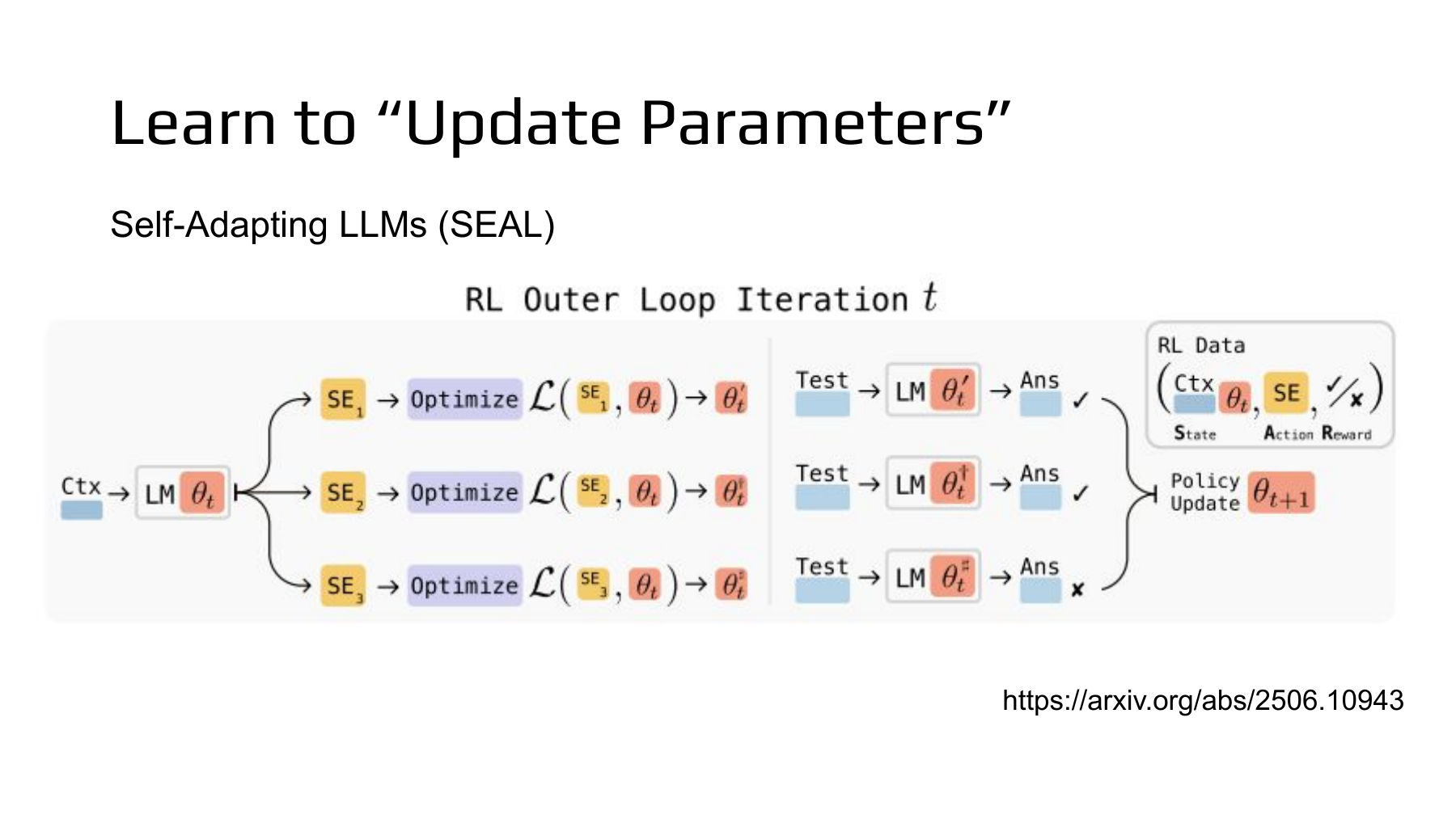
A single line on the left splits into three branches. One model has proposed several ways to learn the same task. SEAL (Self-Adapting LLMs) calls each proposal a self-edit (SE). To remember a passage, the model can generate training sentences derived from it. For an ARC task involving colored grids, it can specify how to rotate or reflect examples, which learning rate to use, and how many epochs to train. NTU lecture at 40:22 · SEAL paper, examples of both kinds of edit
Follow one branch. The current model θₜ reads context C and writes edit eⱼ. Supervised fine-tuning (SFT) applies the edit to a copy starting at θₜ and produces weights θ′ⱼ. That copy solves a query held out from the demonstrations. Its answer is checked against the target. The inner update changes the copy that solves the query. The outer update uses the result to train the model that will propose future edits. To construct θₜ₊₁ on the right of the figure, the outer update starts from θₜ. SEAL, Figure 1 · Algorithm 1, lines 4–8
#Worked example 1. What do two successful model copies send back?
In an illustrative grid task, suppose the model samples three edits, numbered 1 to 3, from the same demonstrations. Apply each edit to its own fresh copy. Copies 1 and 2 get every color and position right on the new grid. Copy 3 misses one cell. All candidates in this example meet the same compute budget. Write rⱼ for a reward of one on an exact match and zero otherwise. Here y⋆ is the reference grid and ŷⱼ is the grid predicted by copy j.
Represent the three edits as single-token choices. Given the same input context, let the starting model assign the three choices probabilities pⱼ of 1/2, 1/4 and 1/4 in order. As in Equation 3 of the paper, average over the three samples and hold the reward fixed when computing the negative log-likelihood loss.
The final term is zero because edit 3 earned zero reward. The records returned by copies 1 and 2 pair the input context with a successful edit. The outer model trains to generate those edits. A real edit has multiple tokens, so its log probability is a sum over tokens. The team used ReSTEM, which fine-tunes on selected successful outputs. For ARC, it also excluded configurations that required more than 375 training steps. SEAL, Equations 3–4 · Training budget in Appendix A.2 · Official code selecting successful edits
#Worked example 2. What is the denominator in SEAL’s 72.5% success rate?
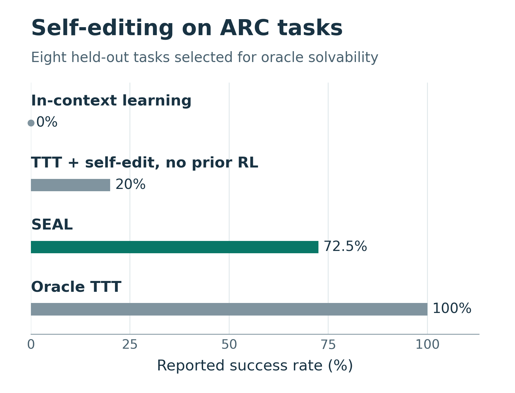
The supplementary chart puts numbers on the check marks in the lecture diagram. The researchers used Llama-3.2-1B-Instruct and selected ARC tasks that the model could solve with a suitable test-time training (TTT) configuration. It learned to propose edits on 11 training tasks. For each of eight separate evaluation tasks, it generated five edits. Each edit was applied independently from the same starting weights. In the two self-edit conditions, a trial therefore means one edit applied to one task. SEAL, experimental setup in §4.1 · Appendix A.3, unit of evaluation
SEAL with outer training succeeded in 29 of 40 trials. Generating edits without that prior training produced eight successes. The difference is 21 trials, or 52.5 percentage points. The five attempts for a given task share its grid rule. The aggregate counts do not tell us how many tasks were solved at least once in five tries. The chart’s 0% is the condition that used only demonstrations in the prompt (ICL). Its 100% is the condition with the human-selected TTT configuration. SEAL, Table 1
Knowledge incorporation uses a different measure. Qwen2.5-7B learned one passage at a time, then answered questions without seeing the passage again. Mean accuracy was 33.5% after training on the passage alone, 39.7% after adding sentences generated before outer training, and 47.0% after adding sentences generated by SEAL. With the single-passage setting held fixed, the difference for the learned generation procedure is 47.0−39.7=7.3 percentage points. During outer training in this experiment, the team evaluated each of five candidate edits per passage with three random seeds and kept the edit with the highest mean score. SEAL, first column of Table 2 · Appendix B.2, selecting edits
#Part II, page 47 — Did the robot improve, or did it learn faster?
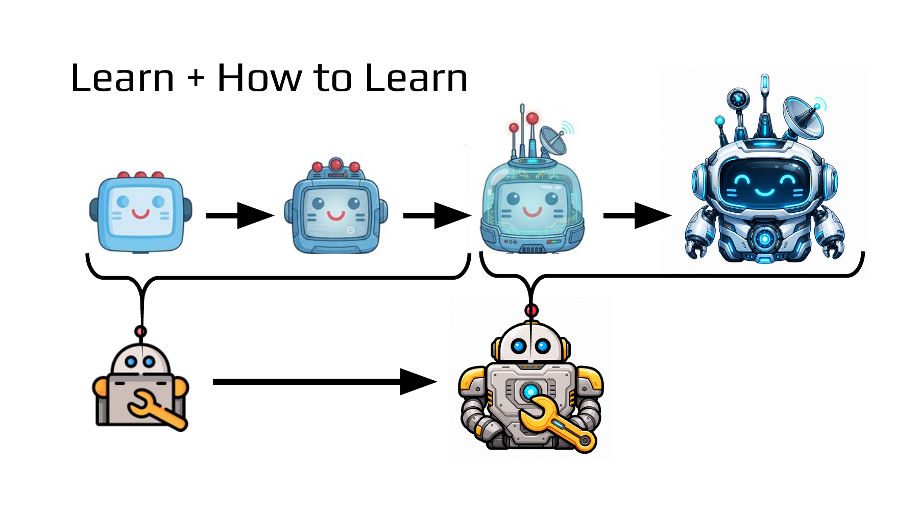
Start with the robots across the top. Each arrow takes an agent from one state to the next. Now look below the braces. A small robot holding a tool sits below each group, and an arrow also connects the two lower robots. The instructor identifies two levels of change. At the top, the agent that performs the task changes. At the bottom, the rule that determines how the agent changes next can change as well. The slide supplies no scores or time scale. A more elaborate robot drawing gives us no numerical estimate of learning speed. NTU Part II, page 47 · Lecture at 42:02
#Worked example 3. Both inspectors finish with 16 correct. Which one learned sooner?
In this illustrative experiment, make two copies of the same initial scratch detector. Update one with rule A and the other with rule B. They receive the same training photos in the same order and have the same compute budget per update. Immediately after each update, score both copies on a fixed set of 20 photos excluded from training. Each entry is the number correct on those same 20 photos.
| Updates completed | Start | 1 | 2 | 3 |
|---|---|---|---|---|
| Inspector trained with A | 10 | 12 | 14 | 16 |
| Inspector trained with B | 10 | 15 | 16 | 16 |
Final accuracy is 16/20=80% for both. If the factory needs the inspector after the second update, A scores 70% and B scores 80%. Let T count the updates needed to first reach 80%. The count cₖ is the number correct after k updates. The minimum selects the earliest update that meets the threshold.
Suppose deployment is equally likely after any of the three updates. Give each post-update accuracy the same weight. The starting model is identical for both rules, and the average here covers the three post-update checkpoints.
B leads by about 8.3 percentage points in mean checkpoint accuracy. The denominator 60 counts 20 photos assessed three times. It does not give 60 independent photos. To evaluate the lower arrow, decide which outcome matters. Does the inspector need the strongest final score after its full budget, or must it reach a usable score sooner? The two questions yield different conclusions from this table.
#Part II, page 48 — What changes within a lifetime and across generations?
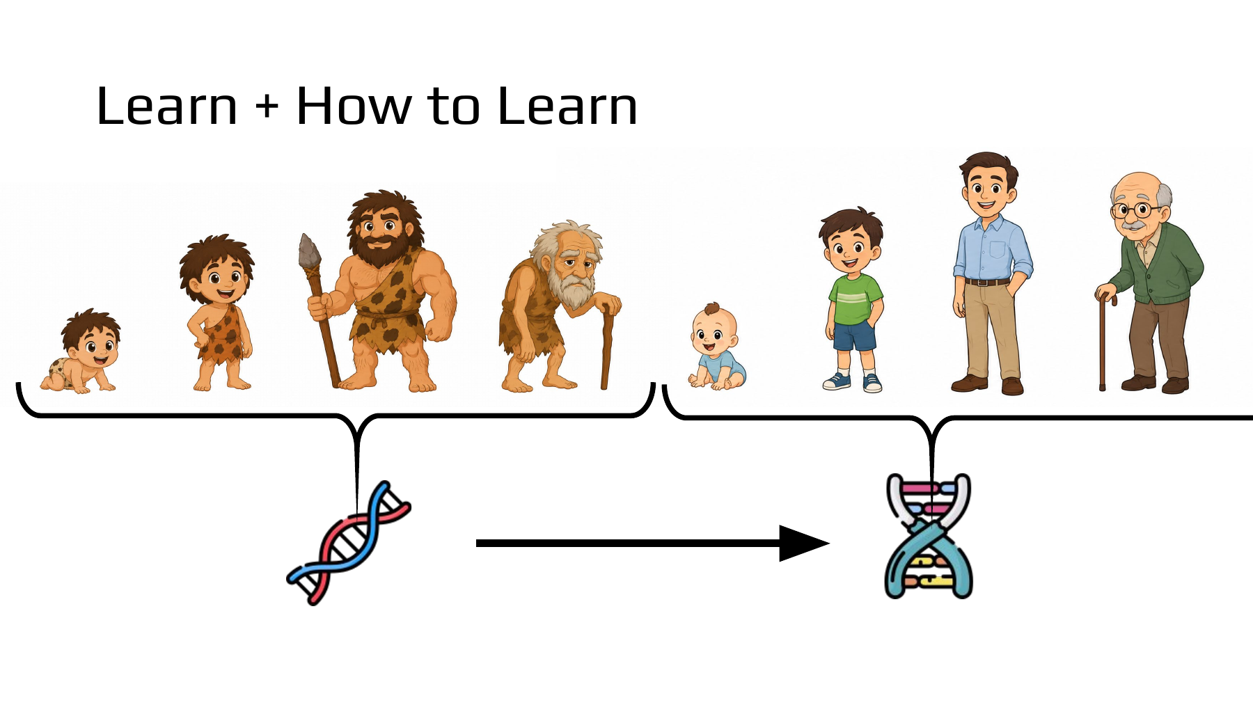
Each brace at the top contains a sequence from childhood to adulthood. Below are two DNA drawings joined by an arrow. The instructor uses this analogy to distinguish changes in brain connections over one lifetime from changes across generations in the distribution of traits that influence learning. In the recorded lecture this analogy follows the notation on page 49. The useful correspondence concerns the two timescales. The picture gives no basis for assuming that a person’s learned memories pass intact to the next generation, or that the group on the right performs better in every environment. NTU Part II, page 48 · Lecture at 44:14
#Worked example 4. What transfers to the next camera: a correction or a calibration method?
Apply the analogy to an illustrative camera calibration experiment. Each new camera starts with its brightness correction θ reset to zero. Measure the brightness offset three times for each device. Rule U uses the most recent measurement as the current θ. Rule V uses the median so far. The table shows the result after both rules have seen all three measurements. An independent reference instrument supplies the offset at that instant. The rules have no access to it. Corrections and errors are in brightness units.
| Camera and condition | Measurements in order | Reference | Correction from U | Correction from V |
|---|---|---|---|---|
| A · stable, noisy final reading | 3, 4, 17 | 4 | 17 | 4 |
| B · stable | −1, −3, −2 | −2 | −2 | −2 |
| C · underlying offset changes rapidly | 1, 5, 9 | 9 | 9 | 5 |
First compare the rules on the stable cameras A and B. Take the absolute difference between the correction and the reference for each camera. Mean absolute error (MAE) averages the two differences.
Under that criterion V wins. What transfers to C is the instruction to use the median of its measurements. C receives neither A’s correction of 4 nor B’s correction of −2. It estimates a fresh correction of 5 from its own readings 1, 5 and 9. On C the ranking reverses.
Rejecting an outlying reading helped on the stable devices. On C the last reading best represented a real change. A method can transfer to a new device, but its performance still needs to be measured there. Page 49 introduces θ and φ for these two levels. The value θ changes while the learner works on a task. The parameter φ specifies how that value gets updated.
#Part II, page 49 — When does θ change, and when does φ change?
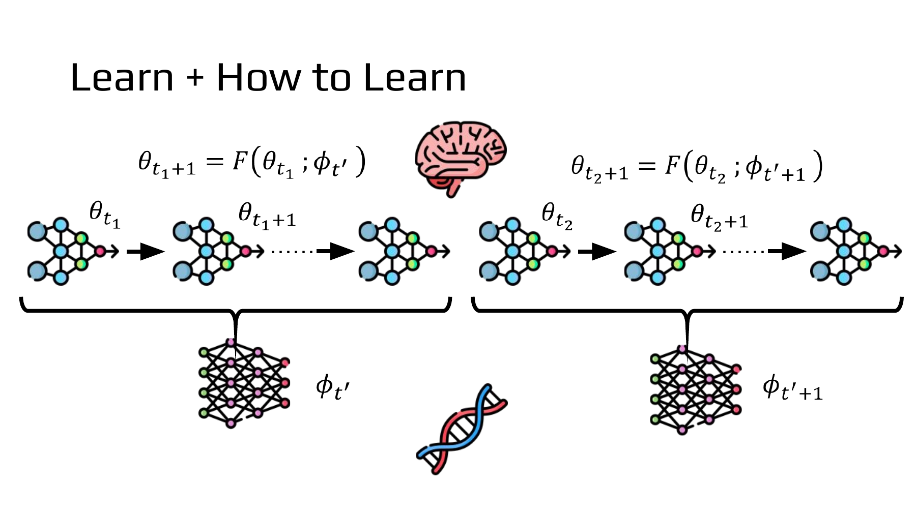
Start with one arrow inside the left brace. The update function F takes the model’s current weights θ and returns the next weights. The parameter φ below the brace determines what F computes. The weights θ can change several times while the same φ stays in effect. The right brace uses a revised learning rule. The subscript t counts inner updates. The index t′ counts updates to the rule itself. Advancing each counter by one can represent very different amounts of work. NTU Part II, page 49 · Lecture at 42:54
#Worked example 5. What do we differentiate to change a learning rate?
Consider an illustrative camera calibration. A small training sample suggests a brightness correction of 2. A separate validation sample suggests 3. Let θ be the current correction and φ the size of a learning step. Fix the starting correction at θ₀=0. For training, use half the squared distance to 2. The starting gradient is −2, so a learning rate of 0.25 gives a correction of 0.5 after one step.
The question changes from “Which way should the correction move?” to “Which step size reduces validation error after one update?” Multiply two rates of change. The validation gradient at the new correction is 0.5−3=−2.5. The updated correction changes by two units per unit change in φ. The outer gradient is therefore −5.
Here 0.05 controls the update to the rule. The resulting 0.50 controls the rule’s update to the model. Starting again from zero and taking the same single step reduces validation loss from 3.125 to 2. Since the validation example helped select φ, a fresh task is needed to find out whether the rule transfers to a new camera.
#Supplementary paper · From a step size to a learned optimizer
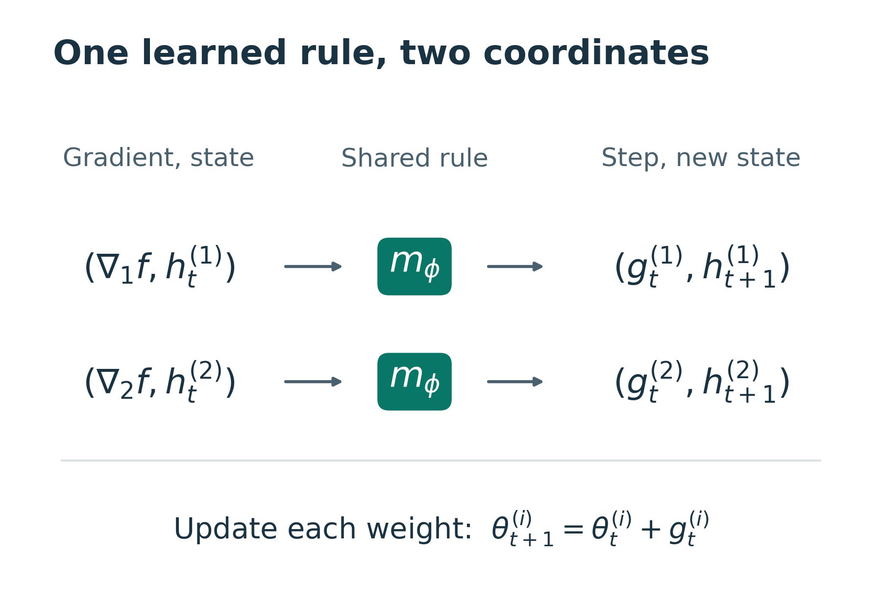
In a 2016 study by Andrychowicz and colleagues, a small recurrent network acts as an optimizer. Given a task gradient and its own previous state, it returns an increment to add to the weights and a new state. The coordinates share optimizer parameters φ but have separate internal states. In the hand calculation, F could only scale a gradient. Here two identical current gradients can produce different updates if the preceding gradient histories differ. Equation 3, updates and training objective · Figure 3, per-coordinate state and shared parameters
How can identical gradients give different updates? Consider a simple momentum rule. Halve the previous accumulator and add the current gradient. With a gradient of 1 for both coordinates but previous accumulators of +2 and −2, the new accumulators are 2 and 0. At a step size of 0.1, the two increments are −0.2 and 0. The coordinates share the rule but carry different histories. This calculation isolates the role of state. The LSTM in the paper can represent a more complex function.
#Part II, page 50 — How do we evaluate meta-learning on a new task?
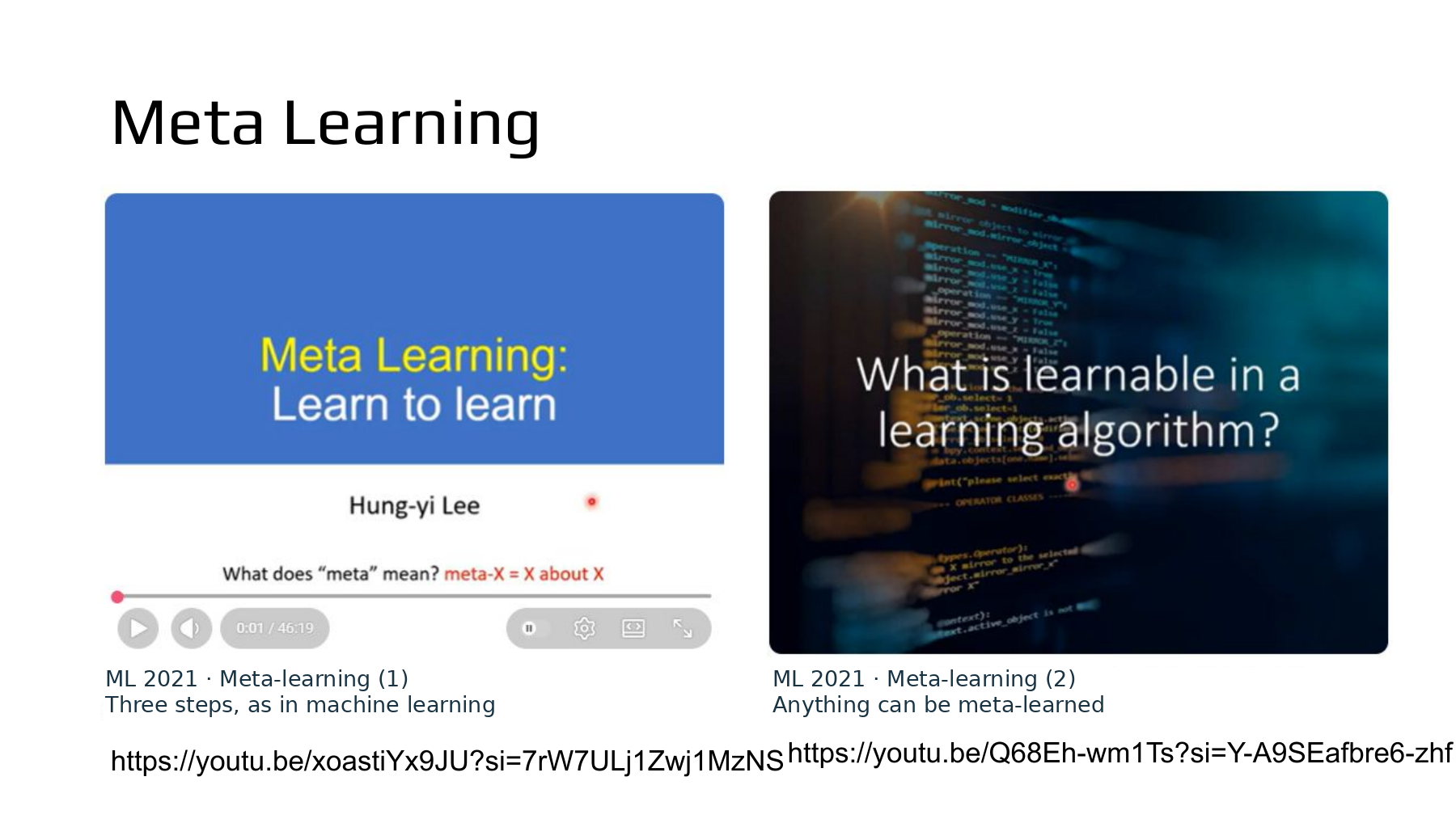
The slide points to two NTU lectures from 2021. The first asks how to score a learning algorithm after it runs on a task. The second asks which part of the learning procedure to learn. Although this slide follows page 49 in the PDF, the instructor introduces the videos before returning to the equation for θ and φ. Main lecture at 42:45 · NTU 2021 course materials
Pause the first video at 19:20 to see the losses from different tasks combined to score a learning rule. Each task contributes a score obtained after learning from its own examples. At 13:20 in the second video, the slide zooms in on the operation that turns a gradient into a weight update. An outer task score can guide different inner choices, including the initial weights, step size or optimizer. First video at 19:20 · Corresponding slide 19 · Second video at 13:20 · Corresponding slide 41
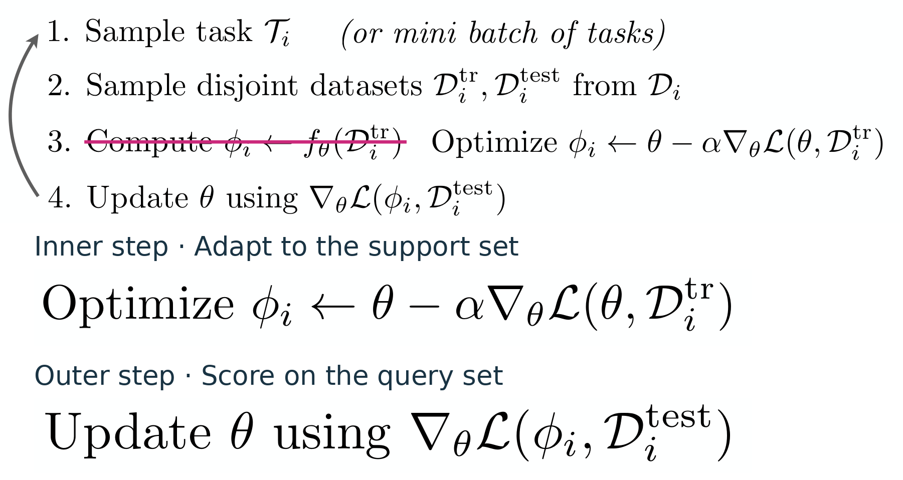
In a task, or episode, shown in the Stanford CS330 lecture, a small support set provides examples for adaptation. A separate query set measures performance after adaptation. During meta-training, query loss supplies the signal for learning the outer parameters. Final meta-testing introduces new tasks that played no part in selecting the learning procedure. There are two splits to keep track of: support and query examples within a task, and training and test tasks across the experiment. Stanford CS330, page 20
#Worked example 6. Which initialization would MAML learn from two cameras?
Model-Agnostic Meta-Learning (MAML) learns initial weights from which a few updates work well on a new task. On page 49, φ parameterized the learning rule. Here the outer loop selects the shared starting value w, while the inner step size stays fixed at α=0.5. Treat cameras A and B as distinct tasks. Let s denote a target correction measured on support images and q a target measured on separate query images. The numbers below are illustrative. MAML, Algorithm 1 · Algorithm 2 for supervised learning
| Camera | Support target s | Query target q | One update from w=0 | Query loss |
|---|---|---|---|---|
| A | −2 | −3 | −1 | 2 |
| B | 4 | 5 | 2 | 4.5 |
Use half the squared error. One update on the support set moves the correction halfway between its starting value and the support target. The query error for A is −1−(−3)=2. For B it is 2−5=−3.
Each query gradient is multiplied by 0.5 because moving the initialization by one unit moves the adapted correction by only half a unit. With an outer step size of 0.4, the new initialization is 0.1. Give the two cameras the same support data again.
Average loss falls slightly, even though A’s error grows. The outer objective selects the starting value using the average across tasks. MAML applies this calculation to many weights. Its choice of initial weights differs both from tuning a single learning rate and from rewarding discrete self-edit text in SEAL.
#Worked example 7. What grows fivefold from 5-way 1-shot to 5-shot?
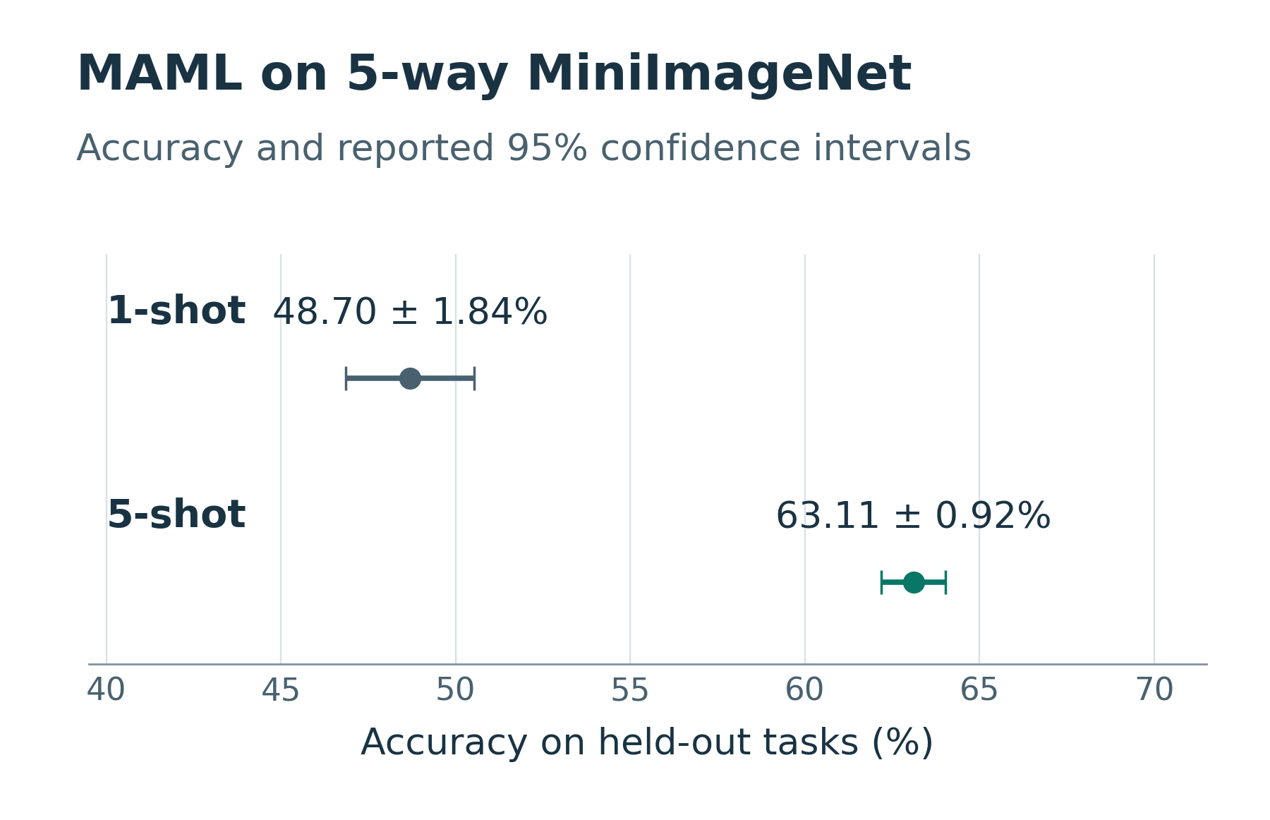
The lower half of Table 1 in Finn et al. reports classification on new miniImageNet classes. 5-way means distinguishing five classes in each task. 1-shot and 5-shot count labeled support images per class. The model therefore sees five or 25 images during adaptation. Accuracy measures how often the adapted classifier predicts a query image’s class. MAML, experimental setup · Table 1, miniImageNet results
The MAML row reports 48.70±1.84% for 1-shot and 63.11±0.92% for 5-shot. 14.41 percentage points is the difference between the reported means. The error bars show a 95% confidence interval over tasks for each mean. The table does not give a confidence interval for the difference itself. In the SEAL experiment a success meant solving an ARC grid after adapting with a self-edit. Here the underlying observations are classifications of new images. Each percentage has to be read in the context of its own task.
Chapter 22 compared training algorithms. We can now say what each method selects and which data score that choice. Page 51 turns to the changing state of a recurrent network as it reads new inputs. Preview of Part II, page 51