An inspection camera says “left” when it sees a yellow part. Give it a one-line routing instruction and it says “right” for the same photograph. Where did that change take place? The weights in the saved model file could be identical before and after. Clear the instruction and start a fresh run, and the answer could revert. Both observations can hold at once.
Chapter 23 asked which learning rule to learn across tasks. Part II, pages 51–55, now asks what that rule writes, and where, during a single sequence. We follow the inner weights of a TTT layer, the neural memory in Titans, and the values a Transformer retrieves from context. The tokens, cameras and routing instructions used in the calculations are teaching examples.
Worked examples Writing and reading a token · Token order and loss · KV cache size · Surprise and forgetting · Memory update rates · Testing retention · Reading a changed rule
Video timestamps by slide
| Part II slide | Lecture video | What to look for |
|---|---|---|
| Page 51 | 45:47 | A hidden state represented by the weights of a small model |
| Page 52 | 47:34 | An earlier lecture comparing RNNs, Transformers and Mamba |
| Page 53 | 47:54 | What changes within Titans and Nested Learning as inputs arrive |
| Page 54 | 48:42 | What a change in behavior can tell us |
| Page 55 | 50:25 | Why Lee compares the hidden state to a brain and slower weights to genes |
Each link opens the point where Lee discusses the topic. Time runs from left to right in the diagram on page 51. The 2025 lecture linked on page 52 is a separate recording. NTU course schedule, May 22, 2026
#Part II, page 51 — Which numbers change as a model reads a token?
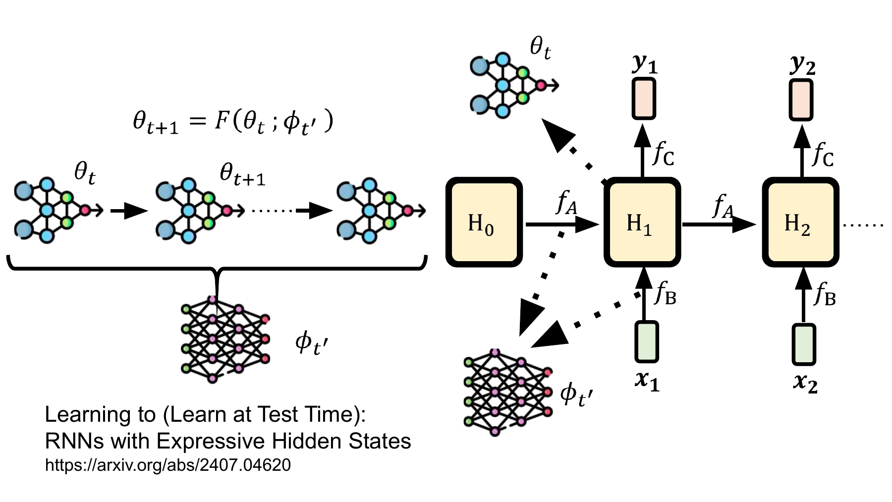
Start at the bottom of the diagram on the right. The first token x₁ enters through f_B. The initial hidden state H₀ enters from the left through f_A. Their paths meet at H₁. The function f_C reads that state to produce y₁. When x₂ arrives, the same functions produce H₂ from H₁ and x₂. Lee maps the fast parameters θ from the previous slide to the contents of these boxes, and the slower parameters φ to the functions that govern them. One set of numbers changes as a sentence unfolds. The other determines how to read many sentences. Lecture at 45:47, introducing the paper · At 46:46, interpreting H as parameters
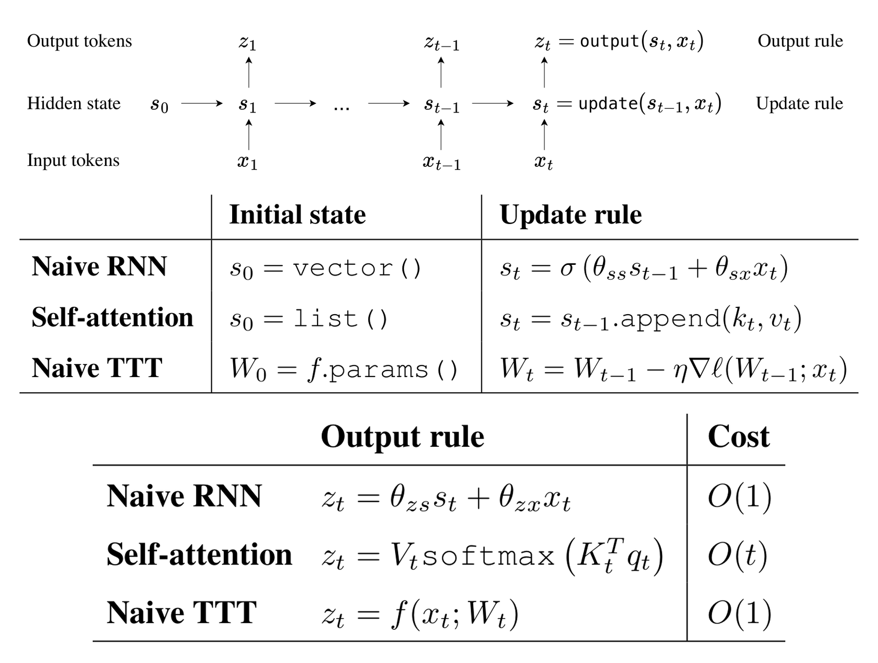
Sun and colleagues give this interpretation a concrete implementation. They use the weights W of a small predictor as the hidden state. Read the three update rules in the middle panel. A simple recurrent neural network (RNN) changes its state vector. Self-attention appends a key and a value to a list. A test-time training (TTT) layer subtracts a loss gradient scaled by a learning rate from W. The output equations in the lower panel show how each layer reads its updated state. Lee’s analogy applies across the rows. The TTT row explicitly builds a self-supervised gradient step into the forward pass. ICML 2025 paper, Figure 2
#Worked example 1. What does one token write to the weights, and what does it read?
Equations 3 and 4 in the paper project the current token representation xₜ into three views. The key kₜ supplies the input to the small predictor. The value vₜ supplies the target features to reconstruct. The query qₜ supplies the features used to read the updated predictor. All three come from the current token, so the layer can take its inner step before the next word arrives. The outer loop learns the three projection matrices. Paper, Equations 3–4
For a calculation by hand, make the small predictor a single multiplication, f(k; w)=wk. Scale the squared reconstruction error by ½ so that the factor of two cancels in its derivative. Start with weight 0 and learning rate η=½. Suppose token A supplies (k,v,q)=(1,2,2). Its prediction before the update is 0 and its target is 2.
The last line measures reconstruction on the key, 1, then reads the layer output z₁ on the query, 2. The output is a feature that travels onward through the network. The language model still has to turn it into a distribution over next tokens. We have left out bias and normalization and evaluated a fresh gradient for each token. The paper also introduces mini-batches of tokens so a device can evaluate several gradients in parallel. Paper, §2.4 and Figure 3
#Worked example 2. Can two tokens in a different order change the next-word probability?
Give token B target −2 and keep the key at 1 and the query at 2 for both tokens. Restart at w₀=0 for each sequence, then use the same update as above. Each new weight lies halfway between the previous weight and the incoming target.
| Reading order | After writing the first token | After writing the second token | Final output z₂=2w₂ |
|---|---|---|---|
| A → B | 1 | (1−2)/2 = −0.5 | −1 |
| B → A | −1 | (−1+2)/2 = 0.5 | 1 |
Now build a toy language model with two possible next words. Assign z₂ as the logit for word C and set the other word’s logit to 0. Suppose the correct next word happens to be C for both sequences. Applying softmax gives the probability assigned to C. Its negative natural logarithm gives the next-token loss.
The later target has a larger influence on the final w. The inner loss ℓ scores reconstruction of v from the current token. The outer loss L scores the probability given to the actual next word after the layer has stored that context. During training the outer loss teaches the projections and the rest of the language model how to use this memory. At deployment the layer can update W for a new sentence from the tokens of that sentence alone. Paper, §2.2 on the two learning loops
#Part II, page 52 — Which memory grows as the sentence gets longer?

This slide points to Lecture 4 of NTU’s 2025 machine learning course. It compares how RNNs, self-attention and Mamba carry earlier information to a later position. Page 51 asked how to interpret H. Watch the companion lecture with a more concrete question in mind. Which numbers from earlier tokens does the model carry forward so it can process the next one? Current lecture at 47:34 · 2025 lecture video · Companion slides, pages 10–11
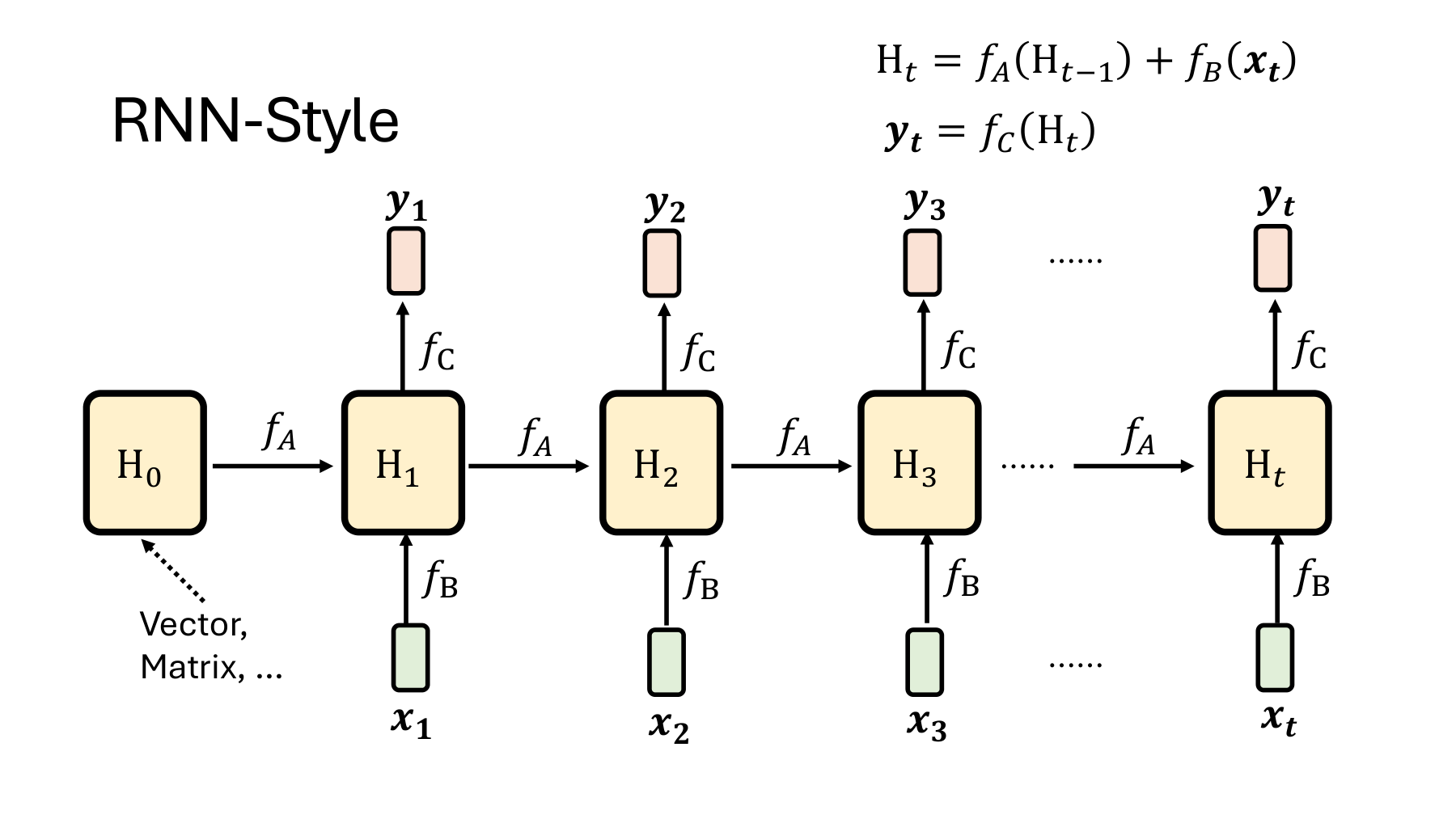
On page 11 of that deck, H₁ is computed from H₀ and x₁. When the layer computes H₂, there is no direct arrow from x₁. Its contribution travels through H₁. Page 17 traces a different route. A new query forms a dot product with each available key. Softmax turns the scores into weights for the corresponding values. Keeping the earlier keys and values available for this operation gives us the key–value (KV) cache. 2025 lecture at 12:30, tracing the recurrence · State update, page 11 · Self-attention, page 17
At 46:00 the same lecture derives linear attention, which accumulates keys and values into one matrix. The linear formula on that slide can combine many positions during training and update a matrix recurrently during inference. Page 17 uses softmax on its scores. The storage comparison below uses full self-attention as shown on page 17. 2025 lecture at 46:00 · Companion slide 40
#Worked example 3. What do we store and read at token four and token eight?
Take one attention head with two numbers per key and two per value. Each position can attend to every earlier position and itself. Just before producing the output at position t, the cache holds t pairs. The current query scores each key once. For comparison, give our linear TTT layer a single bias-free matrix W that maps two-dimensional keys into two-dimensional values.
| Current position | Numbers in the KV cache | Query–key dot products at this position | Numbers in the linear TTT state W |
|---|---|---|---|
| Token 4 | 16 | 4 | 4 |
| Token 8 | 32 | 8 | 4 |
TTT has its own cost for updating W and computing Wq at each token. The table counts state carried across positions and keys scored by a query. Wall-clock time and total GPU memory also depend on the layer width, model weights, temporary arrays and parallel execution. A fixed-size state compresses the past. For instance, under our scalar update, target sequences (2,−2) and (0,−1) both leave a final weight of −0.5. Reading that weight alone cannot recover which pair occurred. The paper’s long-context experiment evaluates the information that survives compression by measuring perplexity on next-token prediction. Lower perplexity means a higher geometric mean probability for the observed next tokens. On the right of Figure 1, under matched training compute, TTT-Linear and TTT-MLP keep reducing perplexity beyond 16k tokens of context. The Mamba curve stops improving in that experiment. TTT paper, long-context experiment in Figure 1 · State and computational cost in Figure 2
#Part II, page 53 — What does Titans store, and when does Nested Learning write?
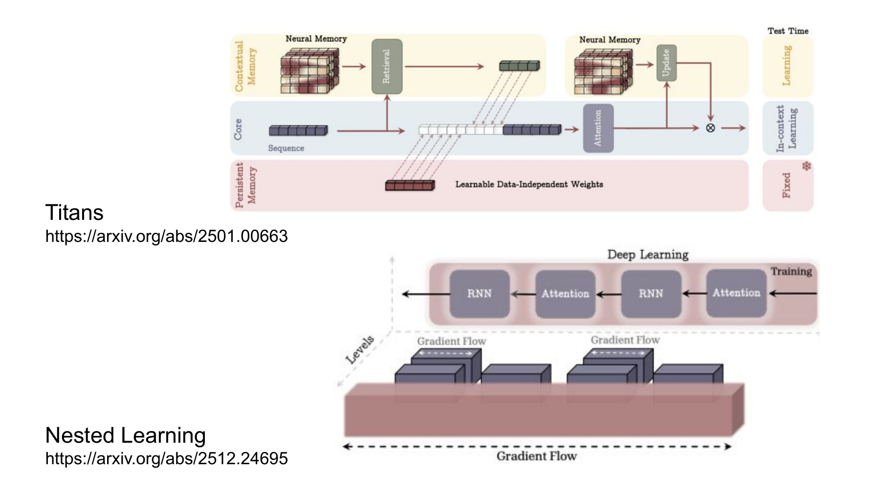
The upper diagram shows one of the three Titans designs, memory as a context (MAC). When a segment arrives, the model retrieves information from its neural memory. The attention block in the middle reads that information alongside the current segment and the learned vectors at the bottom. Its output helps update the neural memory for the next segment. This explains the two labels on the right. The persistent memory at the bottom consists of input-independent vectors learned during training. The contextual memory at the top changes as the model reads. Lee uses these two papers to ask which quantities we choose to call a state and which we call trainable weights. NTU Part II, page 53 · Lecture at 47:54 · Titans, Figure 2
#Worked example 4. Why does the previous update matter for the very same token?
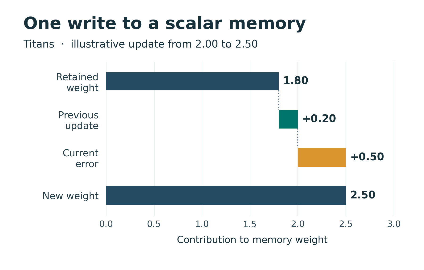
In Titans, surprise has a magnitude and a direction. Each token supplies a key k and a value v. The memory tries to recover v from k. To work through Equation 12, take an illustrative scalar memory that multiplies its key by a weight m. Suppose m=2, the new key is k=1 and the target is v=3. Its output is 2. Increasing m would move the output toward 3. Titans, Equations 11–14
Write S for the previous update and S′ for the new one. The coefficient η carries part of the previous update forward, θ scales the current gradient, and α discounts the old memory itself. In the paper, these coefficients can depend on the input. For this one step, take S=0.4, η=0.5, θ=0.25 and α=0.1.
The bars account for every part of the new weight. The old memory contributes 1.80, the previous update contributes 0.20 and the current error contributes 0.50. Reading the same key now returns 2.5, bringing the squared error down from 1 to 0.25. Dropping only the previous update by setting η=0 gives 2.30. Turning off only the forgetting gate by setting α=0 gives 2.70. The two coefficients act on different quantities. The authors also tested these components separately. Their base neural memory (LMM) scored 92.68% on the long-context accuracy column of Table 5, compared with 87.12% after removing momentum and 85.60% after removing weight decay. These differences describe that particular ablation. Titans, Section 5.9 and Table 5
#Worked example 5. How many writes do three memories make in eight tokens?
Read the lower diagram horizontally and you see RNN and attention layers arranged in sequence. The authors add another axis. Which quantity updates, on what signal, and how often? This is the perspective of Nested Learning. One concrete design, the continuum memory system (CMS), passes each input through several multilayer perceptrons (MLPs). Each block updates its weights at the end of its own token chunk. A block can therefore process a token even when its weights stay fixed for that step. Nested Learning, Figure 2 · Section 7.1, Equations 70–71
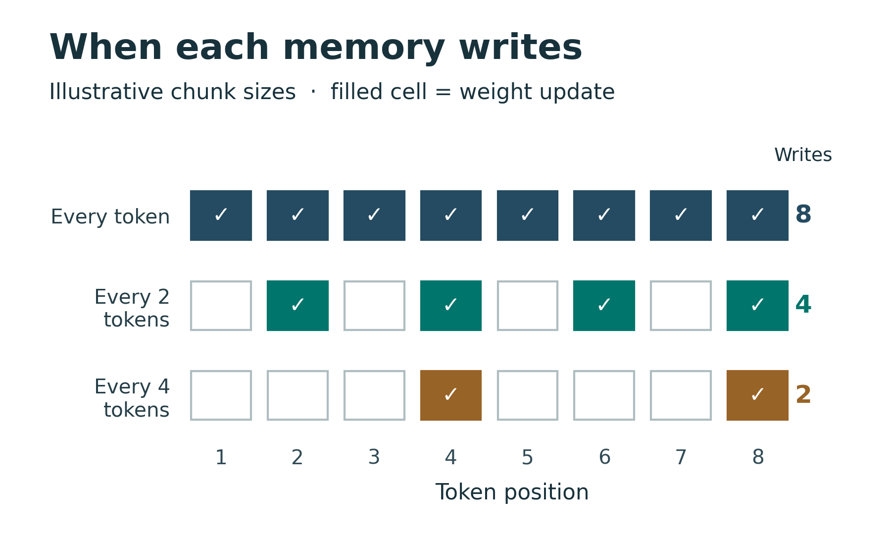
For an illustrative schedule, let the three write intervals C be 1, 2 and 4 tokens. Number the first token 1 and write only at the end of a complete chunk. The number of writes N in a sequence of length T is the number of complete chunks.
All three blocks write after tokens 4 and 8. Only the fastest block writes after token 7. The slowest block still processes token 7 and can produce a different output for it, using the same weights it has held since the end of token 4. A write every four tokens therefore allows an output at every token. The schedule specifies how often weights can change. How long a particular association survives also depends on what was written and how later writes interfere with it. Nested Learning, Equations 70–71
#Part II, page 54 — What can a change in the answer tell us?
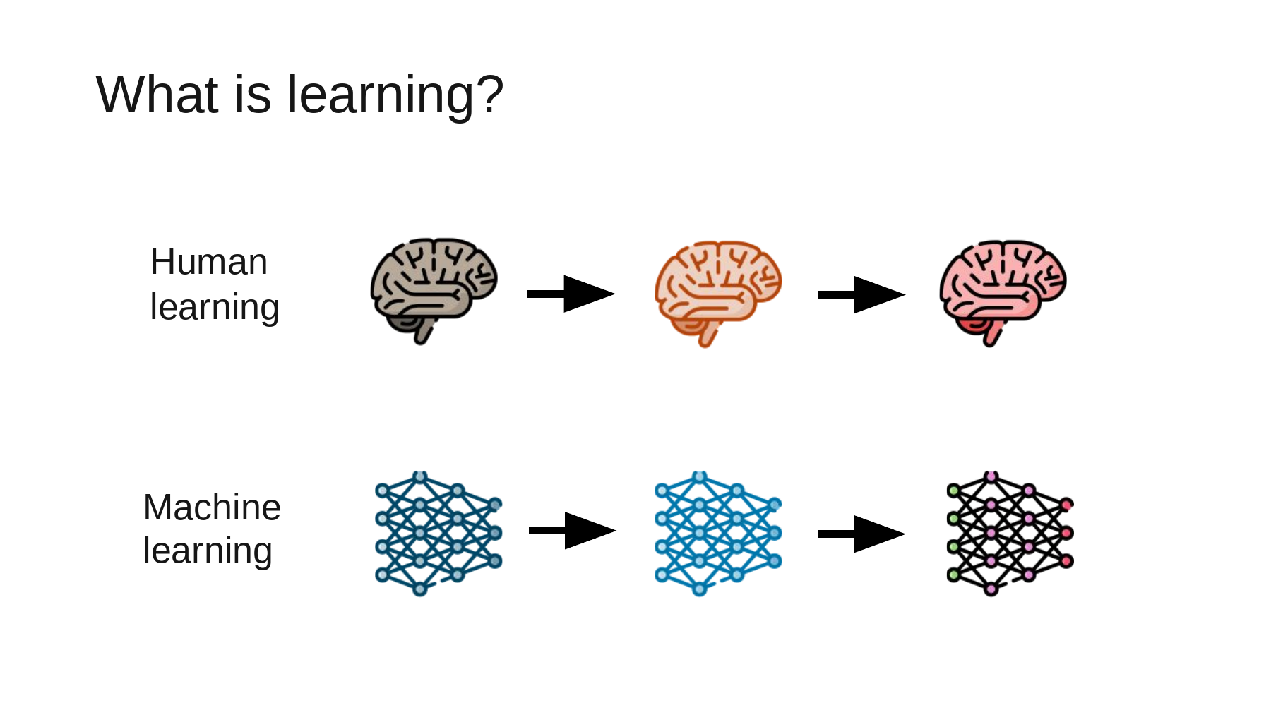
The slide has two rows. In the top row, the brain changes color as a person gains experience. In the bottom row, a network changes color across stages of training. Lee starts with this familiar analogy. It helps separate an observation, “the system changed its behavior,” from one possible explanation, “training changed its weights.” If a model gave a different answer yesterday, we also need to know what information it could read on each occasion. Lecture at 48:42 · The analogy with brain connections at 49:17
Consider a factory where workers reassign the sorting bins between shifts. Today’s instruction says “blue goes left, yellow goes right.” The inspector already recognizes colors. What it needs to learn is which bin goes with which color today. Here we can separate color recognition, which the inspector brings to the shift, from the information supplied by the instruction.
#Worked example 6. How much of the improvement survives a reset?
Take two photographs of blue parts and two of yellow parts. Test each photograph independently. Keep the four images, saved weights, readout rule and correct routes fixed. Suppose the inspector sends everything left before it sees the instruction and routes all four parts correctly while it can read the instruction. For the final condition, restart from the original checkpoint with a fresh context and empty runtime state. The outcomes below are hypothetical.
| Condition on the same four photographs | Two blue parts | Two yellow parts | Correct under today’s assignment |
|---|---|---|---|
| Before receiving the instruction | Left twice | Left twice | 2/4 |
| With the instruction in context | Left twice | Right twice | 4/4 |
| Fresh run from the original checkpoint | Left twice | Left twice | 2/4 |
Subtract the initial accuracy separately from the score while the instruction is present and from the score after the reset. A difference between accuracies is measured in percentage points.
The instruction buys 50 percentage points on these images. The improvement still observable in the fresh run is zero points. The first two rows measure the behavioral effect of having the instruction available. The third tests whether that effect survives this particular reset. If a deployed system can read a conversation log or an external memory, record whether the fresh run can retrieve the instruction again. A real example of adaptation with fixed model weights is Brown et al.’s 2020 GPT-3 evaluation, in which demonstrations in the text specified the task. GPT-3, §2, task presentation
#Part II, page 55 — How can fixed weights follow a new rule?
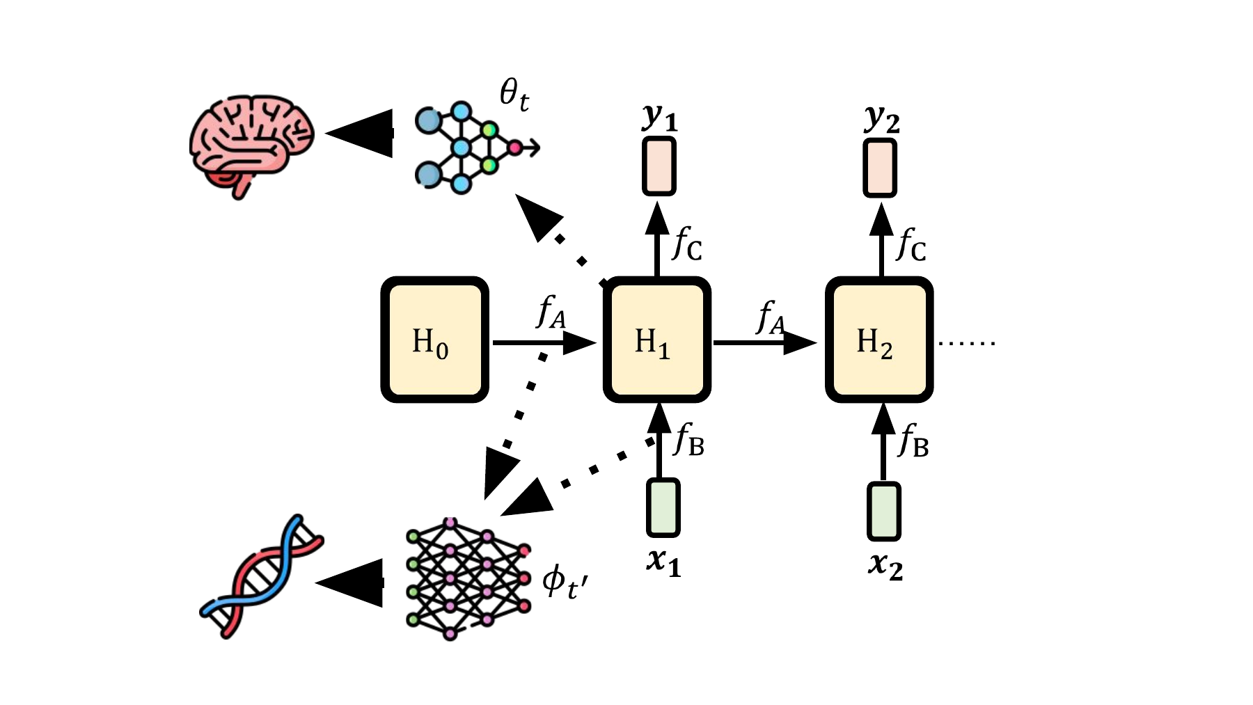
Lee now changes the analogy. On the right, H₀, H₁ and H₂ are successive states as the model reads its inputs. The upper arrow associates the fast-changing state with the brain. The lower arrow associates the outer weights that govern the update with genes. The comparison asks what changes over the course of one experience. The brain and genes serve as an analogy for the two timescales. Lecture at 50:25 · Adding a new rule to context at 51:54
#Worked example 7. Why does the attention output change sign for the same image?
Focus on one blue part. Write the instruction as two entries, one for blue and one for yellow. Suppose the image’s query has scaled scores of ln 3 and zero against their respective keys. The scaling for the key dimension is already included. Softmax exponentiates the scores and divides by their sum. Vaswani et al., 2017, equation 1
The fraction 3/4 is the weight on the blue entry. Encode left as +1 and right as −1, then take the weighted sum of the two values. In this toy representation, colors determine keys and directions determine values. When the next shift swaps the two directions, the query and keys stay the same and the two values change sign.
A fixed readout sends positive values left and negative values right. The same photograph now routes to the other bin. The 0.75 in this calculation weights one instruction entry. It does not give the probability that the chosen route is correct. The calculation used the current values without fitting a matrix. The TTT layer on page 51 implements the dependence on preceding inputs by a different operation, a gradient step on the weights of a small model. Original attention paper, §3.2.1 · TTT paper, §2.3
What observation would distinguish the two mechanisms? On a test that records only the final route, both models could return the correct answer. With access to the implementation, compare the TTT inner weights W before and after one token, inspect the keys and values attention read, and check the saved outer weights separately. Naming the quantity that changed and how long it lasted makes the claim about learning testable. Page 56 follows this distinction through an in-session hidden state, file-backed memory that survives across sessions, and network weights. NTU Part II, page 56