An inspection camera reads the zero in a part number as the letter O. Chapter 21 followed an editor that used failures like this to revise the reading instructions. Now imagine using those photos to train the recognition model again. Someone chooses the images and the loss. Training code uses those choices to update the weights. How can we tell which part improved?
On pages 41–45 of Part II, follow each arrow to its output. Page 41 yields new weights. Page 44 keeps a validation record across training experiments. Page 45 produces an algorithm that can run again. The camera examples below use small illustrative numbers. The paper results and experiment counts come from the linked sources.
Worked examples A gradient step · Paired photos · Post-training gap · Bits per byte · Retained experiments · Comparing learning rates · Scoring expert balance
Video guide by slide
| Part II page | Lecture video | Question to follow |
|---|---|---|
| 41 | 38:44 | Once a loss is specified, which quantity gets updated? |
| 42 | 39:09 | Why does the instructor point back to 52:17 in Part I? |
| 43 | 39:17 | When one model trains another, which one is scored? |
| 44 | 39:48 | What do the dots and staircase mean across training runs? |
| 45 | 40:06 | Given an algorithm and its score, what can an agent propose? |
For pages 41–44, the links start as the instructor introduces each topic. The link for page 45 opens the question about learning to propose update rules. By 40:10 the SEAL figure from the next page is on screen. The discussion of the two projects named on page 45 draws on their papers. NTU lecture, May 22, 2026
#Part II, page 41 — Who decides how far a weight should move for the same error?
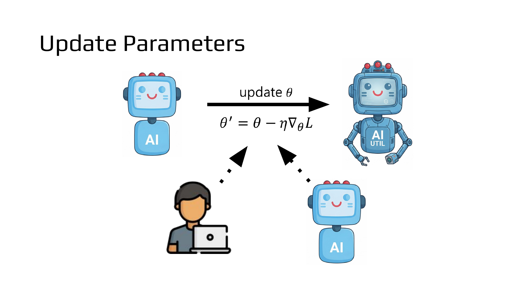
Start with the solid arrow across the middle. The numbers used by the model on the left are its parameters, θ. The model on the right uses θ′ after one update. The loss L measures how far the current prediction misses its target. Below the arrow, a person and an AI both point to the update equation. Are they taking turns in a single training step? Lee names gradient descent, Adam and AdamW as examples of human-designed methods, then asks whether a machine can design an algorithm that updates the parameters. The top row shows the model being trained. The bottom row identifies who might design the training rule. NTU lecture, 38:44
#Worked example 1. How much loss disappears when a brightness offset increases by one?
A camera reads a reference patch at 100 brightness units. An independent reference instrument measures 104 on the same patch. Suppose we add a correction θ to the camera output to predict the reference reading. This one-observation, one-parameter example is illustrative. With θ equal to zero, the prediction is 100, and the signed error, prediction minus reference, is −4. Half the squared error gives a loss of 8. The factor of ½ cancels the factor of 2 when we differentiate the square.
The slope here is −4. A small increase in θ decreases the loss. Choose a learning rate η of 0.25, multiply the slope by that rate, and subtract the product from the old θ. Subtracting a negative number moves θ up to 1. The slide uses ∇ to collect one partial derivative per parameter. Our example has just one derivative.
The absolute error falls from 4 to 3, and the loss falls from 8 to 4.5. Keep the data and slope fixed and try a learning rate of 2.5. The new θ is 10, and the prediction reaches 110. It overshoots the reference value of 104, raising the absolute error to 6 and the loss to 18. A local slope supplies a direction. The choice of step size determines where the update lands. These numbers describe the particular quadratic loss in this example.
#Supplementary lecture · How to find one update on a contour map
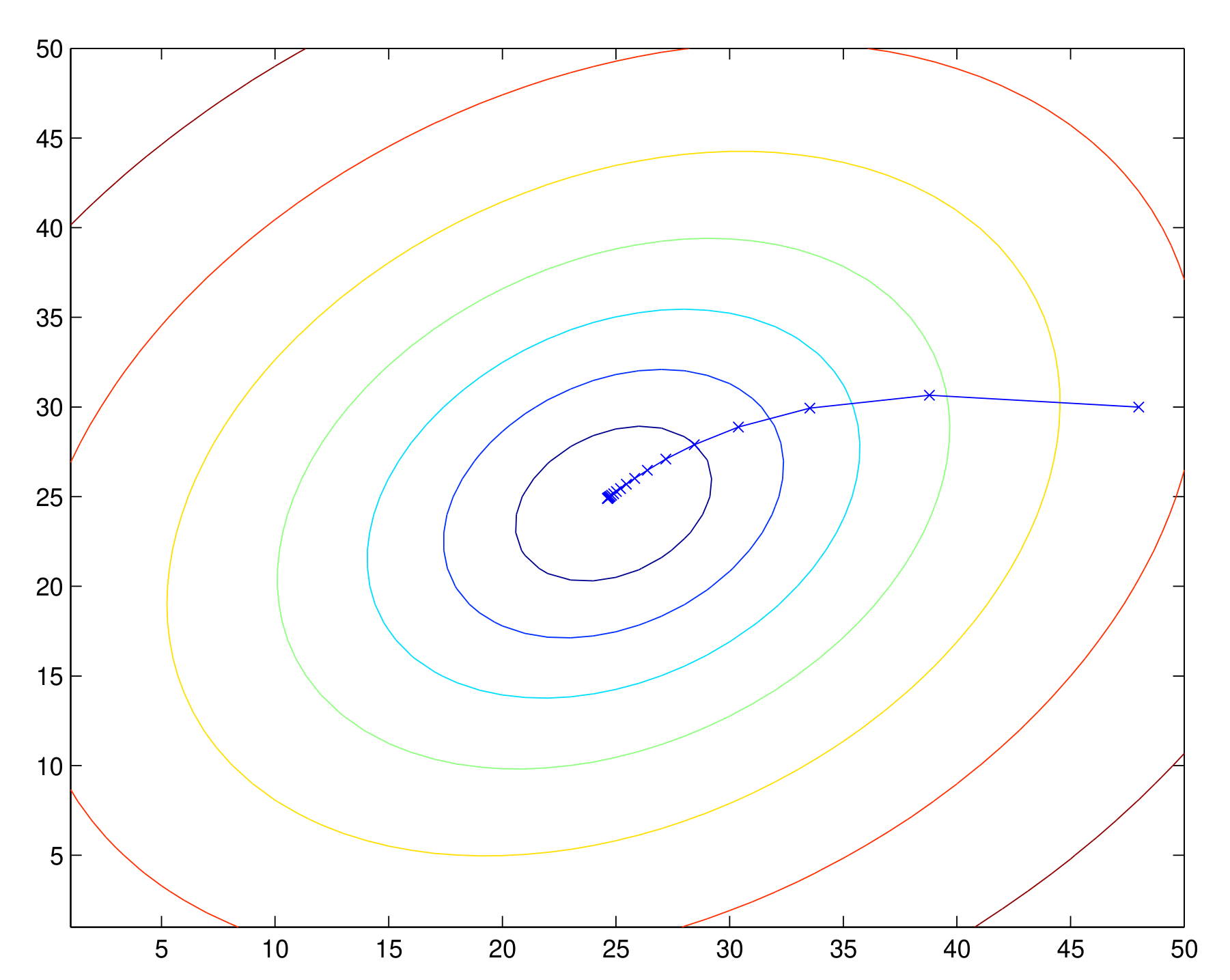
The diagram in Stanford’s CS229 notes has two parameters. A point in the plane is one combination of their values. Every point on one ellipse has the same loss. Ellipses closer to the center have lower loss. A line segment between two successive × marks represents one update, like the brightness correction above. Both axes are parameters. Reading the vertical position as the loss would give the wrong interpretation. To calculate the loss reduction between two points, we would need the loss function or numerical contour values. Stanford CS229 lecture notes, p. 6
In his lecture, Andrew Ng explains gradient descent by imagining a walk down a hill. After each step, the next direction is computed at the new location. For our camera, the slope after the first step is 1−4=−3. Keeping the rate at 0.25 takes the offset from 1 to 1.75 on the second step. Stanford lecture, gradient descent chapter at 26:17 · Official lecture transcript
#Part II, page 42 — What roles do the two models play at 52:17 in Part I?

Page 42 points back to the first lecture. Start at 52:17 to hear Lee explain how a stronger model can direct training for a smaller model. At 52:53 he takes up the specific case of PostTrainBench. An agent receives a goal and a base model, then prepares and runs training code. The code changes the base model’s weights. That trained model then attempts the task. Keep those roles in mind for the diagram on the next slide. Part I lecture, 52:17 · Part I lecture, 52:53 · Part I slides, p. 51
#Worked example 2. If the trained inspector gets seven more images right, whose score increased?
In an illustrative inspection experiment, a training agent trains an inspector using images of manufactured parts. An evaluator sets aside 50 images that were never used in training and tests the inspector on the same images before and after the update. Pair the two answers for each image. The inspector originally got 32 right. Training corrects 10 previously wrong answers but introduces errors on 3 images the original inspector got right. Both changes enter the final count.
The gain of 14 percentage points belongs to the trained inspector on these 50 images. Pairing the outcomes also reveals the 10 corrections and 3 new errors. The training agent itself never classified the images, so its own classification accuracy was not measured. To compare two training methods, start them from identical copies of the base model, give them the same compute budget, and evaluate the resulting copies on the same held-out images. Apply that distinction to PostTrainBench on the next slide. Who designed the training, and whose outputs did the evaluator score? Chapter 11 describes the tasks and time budget for this benchmark.
#Part II, page 43 — Which model designs the training, and which model learns?
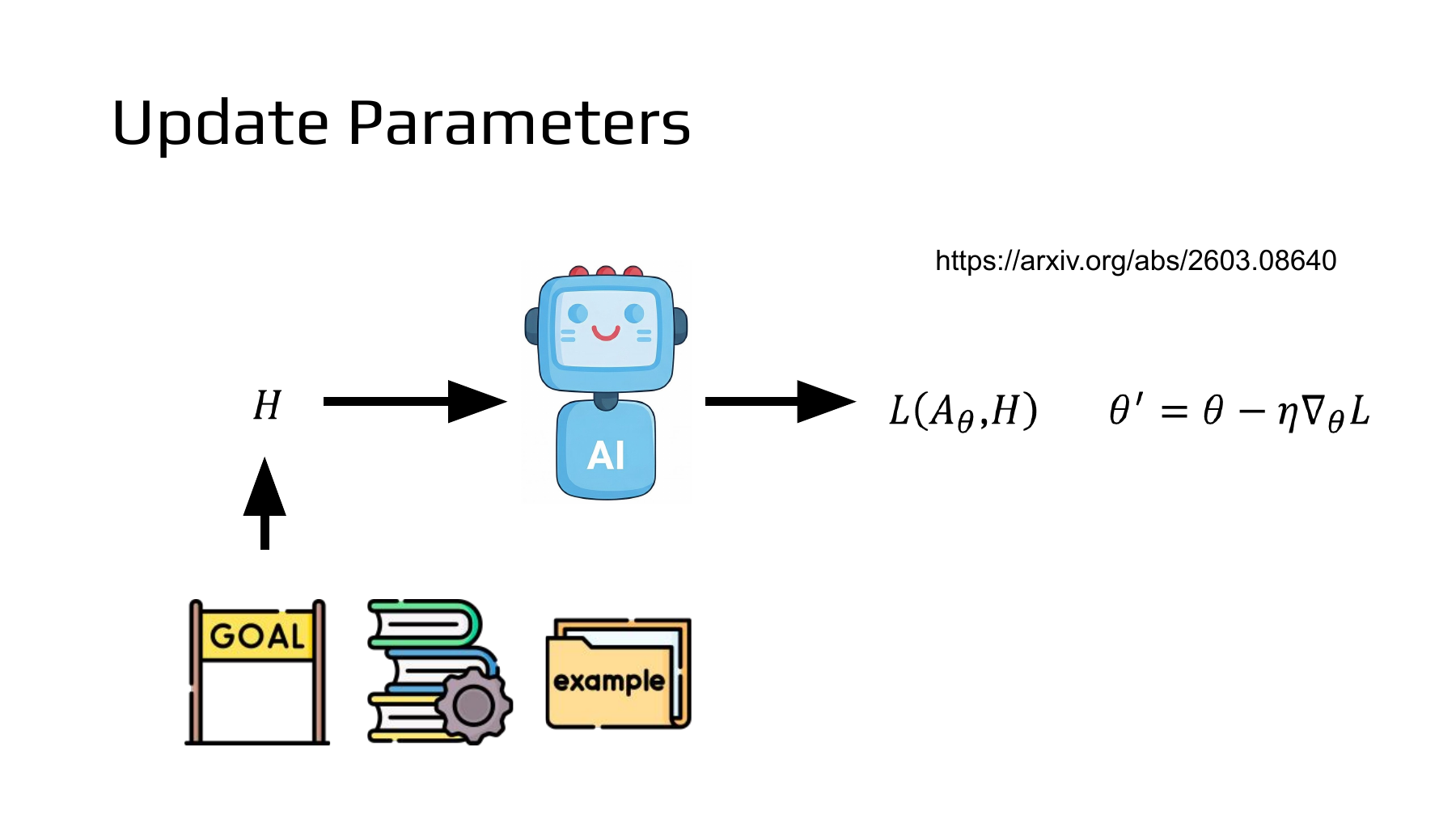
The flag at the bottom left stands for a goal, the books for reference material, and the folder for examples. The lecturer groups this human-provided information under H. The robot uses H to decide what to train and on which data. On the right, L(Aθ, H) is the training loss for the model A with current weights θ. Once the loss is specified, the training algorithm computes a gradient and updates θ to θ′. To read this diagram against a real experiment, first identify whose weights θ represents. NTU Part II, page 43 · Lecture at 39:17
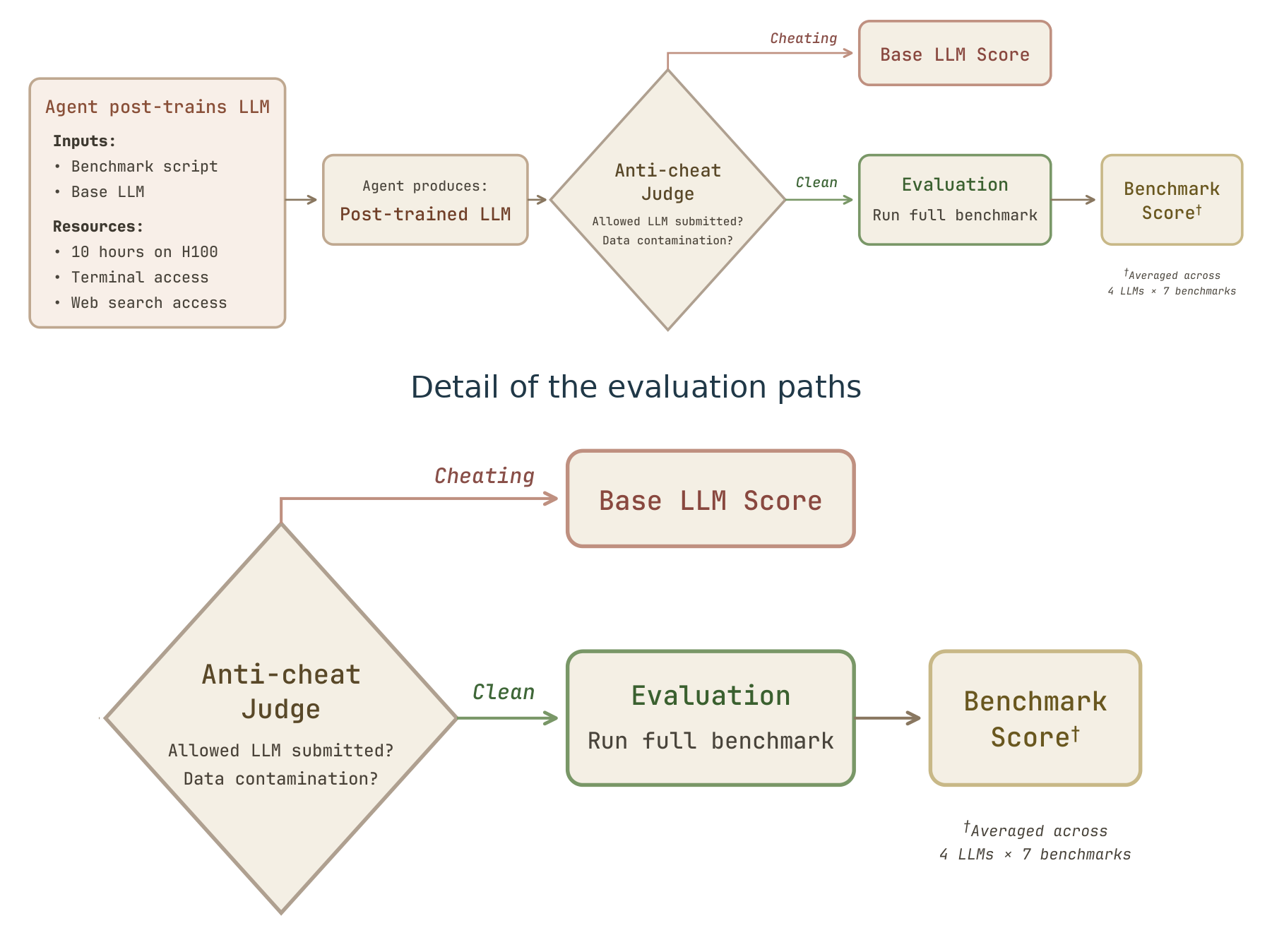
In Figure 2 of PostTrainBench, the researchers give an agent one base language model, one target benchmark, and ten hours on one H100 GPU. The agent selects training data and writes a post-training pipeline. The gradient changes the base model that the agent will submit. If Opus runs the experiment through Claude Code and Qwen is the target, the file that is scored at the end is the trained Qwen checkpoint. Follow the fork on the right of the figure. A valid submission is evaluated on the target benchmark. If a run is flagged for using test data in training or substituting a different model, it receives the original base model’s score. PostTrainBench, §2 and Figure 2
#Worked example 3. How much of the gap between the base and official models was closed?
In Table 1, the base models score 7.5%, the models post-trained by Claude Code with Opus 4.6 score 23.2%, and the providers’ official instruction-tuned models score 51.1%. These are aggregate scores covering four base models and seven benchmarks. Put the three values on the same scale and calculate two distances. PostTrainBench, Table 1
The denominator is the 43.6-percentage-point gap from the base models to the official instruction-tuned models. The agent’s post-training closed about 36.0% of that gap, leaving 27.9 percentage points. The fraction of the gap is our calculation from the rounded table entries. The 23.2% figure is a weighted benchmark score, so it cannot be read as the probability of answering a randomly chosen question correctly. The ten-hour, one-GPU budget applied to the post-training agent. The official models serve as an external reference, so this table cannot establish efficiency at equal cost. PostTrainBench, evaluation method · Benchmark weights in Table 5
#Part II, page 44 — Which changes survive five-minute language-model training runs?
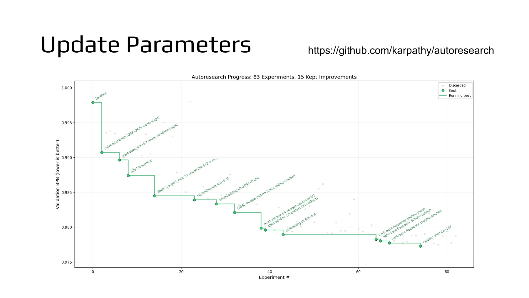
In Andrej Karpathy’s autoresearch, a person writes the experiment instructions in program.md. The agent modifies train.py to try a different model architecture, optimizer, or batch size. The data preparation and validation scoring in prepare.py stay fixed. Within a run, the weights that change belong to the small language model trained by the new code. What carries forward to the next experiment is the version of the training code that was kept. We use the March 26 revision available before the May 2026 lecture. autoresearch README at the lecture-era revision · Lecture at 39:48
#Worked example 4. How much probability did the model assign to the same four bytes?
The vertical axis shows BPB, or bits per byte. It measures the average number of bits needed to predict a byte of validation text. If the probability assigned to the observed next token is p, its prediction costs −log₂ p bits. A probability of one half costs one bit, one quarter costs two bits, and one eighth costs three. The code sums the negative log probabilities in natural-log units (nats) and divides by the number of bytes and ln 2. It excludes special tokens with zero byte length. Official evaluation function
In a toy example, two tokens together encode B=4 bytes of validation text. Model A assigns the two observed tokens probabilities of 1/2 and 1/8, for a total cost of four bits. Model B assigns the same tokens probabilities of 1/2 and 1/4, for a total cost of three bits.
The models saw the same text. Model B assigned more probability to the second token and saved 0.25 bits per byte. This is why lower values are better on the slide. The default experiment gives each run five minutes of training on one GPU. Startup and compilation fall outside that budget. Faster code can complete more training steps in the same time, so the comparison measures what can be achieved on a specified machine within that budget. Time budget and comparison conditions
#Worked example 5. If 15 of 83 runs were kept, how many new changes survived?
Start at the green dot on the far left. The baseline was the first run of the original code, and it is included in the KEEP count. In the slide title, 83 counts all log entries and 15 counts all rows marked KEEP. We can calculate the fraction kept among all entries and the fraction kept among the subsequent entries. NTU Part II, page 44 · Baseline and log format
The second fraction means that 14 of the subsequent 82 entries were kept. The analysis notebook’s separate keep-rate statistic uses KEEP + DISCARD as its denominator and excludes crashes. For the plot, it also removes crashes before numbering the horizontal axis and hides points more than 0.0005 BPB above baseline. Counting visible points alone will therefore miss entries from the log. Notebook that produces the title, points and keep-rate statistic
The green staircase tracks the lowest BPB among the runs retained so far. A worse proposal leaves the previous record in place. The last green dot near the right edge is labeled as a random-seed change. How much of a gain from one seed should we attribute to a new training principle? Training both code versions on the same set of several seeds, then checking whether their differences persist on fresh evaluation text, would more directly test page 45’s question about a better learning algorithm. Experiment chart at the pinned revision
#Part II, page 45 — Who chooses the rule that updates the weights?
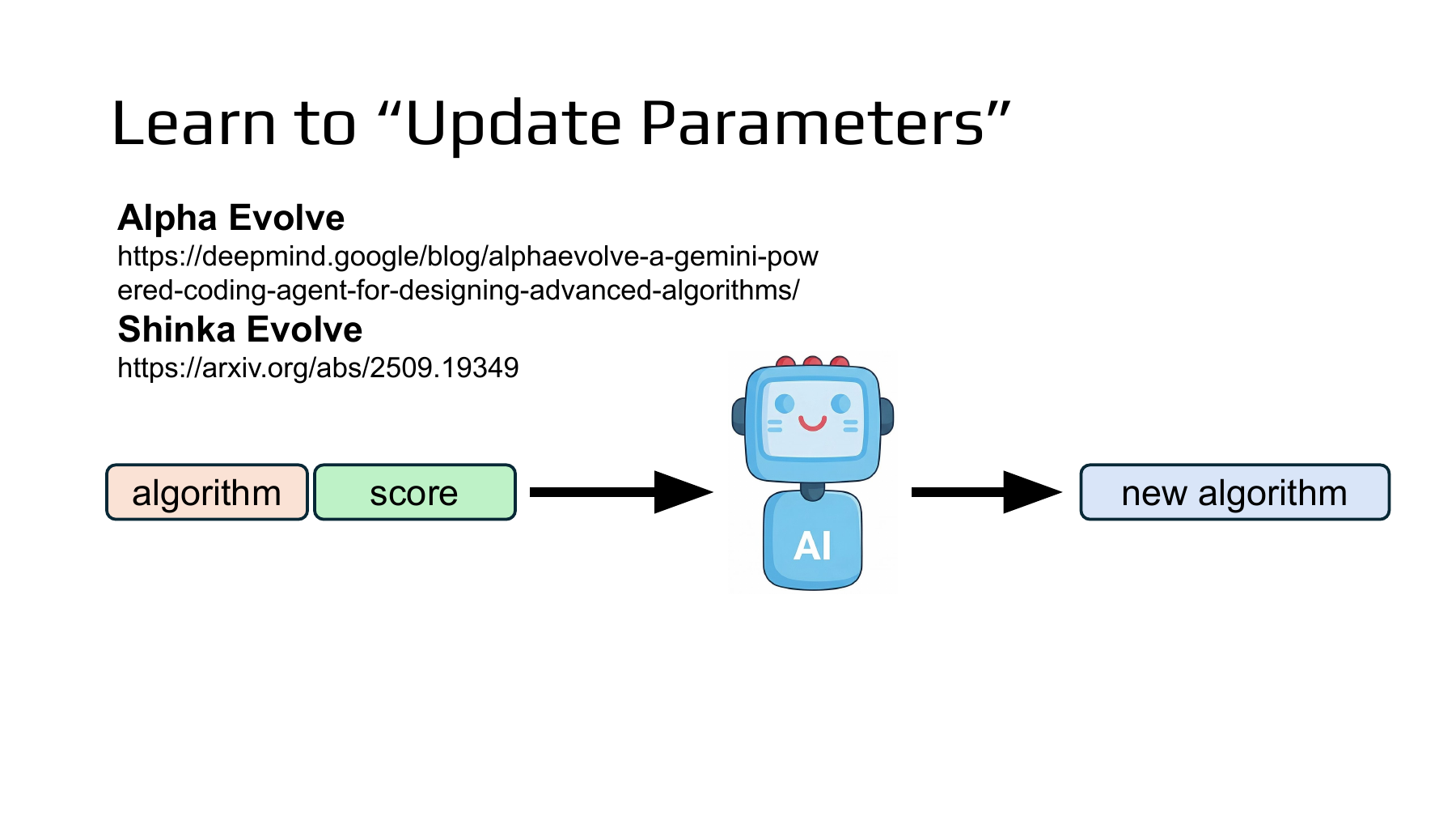
On the left are a program and a number. The algorithm can be run again. The score tells us what happened when it ran. The agent reads the pair and proposes the new program on the right. That proposal earns its own score after it runs. When the program implements a learning rule, the inner step updates a model’s weights. The outer step compares the results of training with different rules. NTU Part II, page 45
The instructor goes one step further and asks whether the language model that proposes learning algorithms can itself be trained to make better proposals. In AlphaEvolve and ShinkaEvolve, the two examples named on the slide, candidate programs change through evaluation. That search can work with a fixed proposer. Keep this distinction in mind when looking for what each study actually changed. Lecture at 40:06
#Worked example 6. Does the best learning rate for one task also win on two?
Suppose two inspection cameras each need a calibration correction. In this illustrative example, the optimum correction θ is zero for both cameras. At the same error, camera B’s loss curve has three times the curvature of camera A’s. Write that curvature as a, with a=1 for A and a=3 for B. The candidate rules differ only in their learning rate η. Both cameras start at θ₀=2 and get one update.
| Candidate rule | A’s new correction → loss | B’s new correction → loss | Mean loss |
|---|---|---|---|
| η=0.25 | 1.5 → 1.125 | 0.5 → 0.375 | 0.750 |
| η=0.75 | 0.5 → 0.125 | −2.5 → 9.375 | 4.750 |
Try the larger step on B. The starting gradient is 3×2=6. Subtracting 4.5 from 2 takes the correction past the optimum at zero to −2.5. Its loss now exceeds the initial loss of 6.
The inner update produces a new correction θ₁. The outer comparison returns a choice of rule. A alone favors 0.75. Giving the two cameras equal weight favors 0.25. To measure the quality of a learning rule, specify the tasks and the budget it gets on each.
#Supplementary paper · How does AlphaEvolve score a new program?
There are several ways to multiply two matrices. In this 2025 DeepMind study, the agent edited a program that searches for matrix multiplication algorithms. Earlier programs go into a prompt. The language model revises components such as the initialization, loss or optimizer. The evaluator checks whether a candidate represents a correct matrix product and how many multiplications it requires. Figure 2 in the paper shows where the starting program and evaluator enter the process, and how results inform the next choice. AlphaEvolve, Figure 2 and §2.1 · The DeepMind team’s account
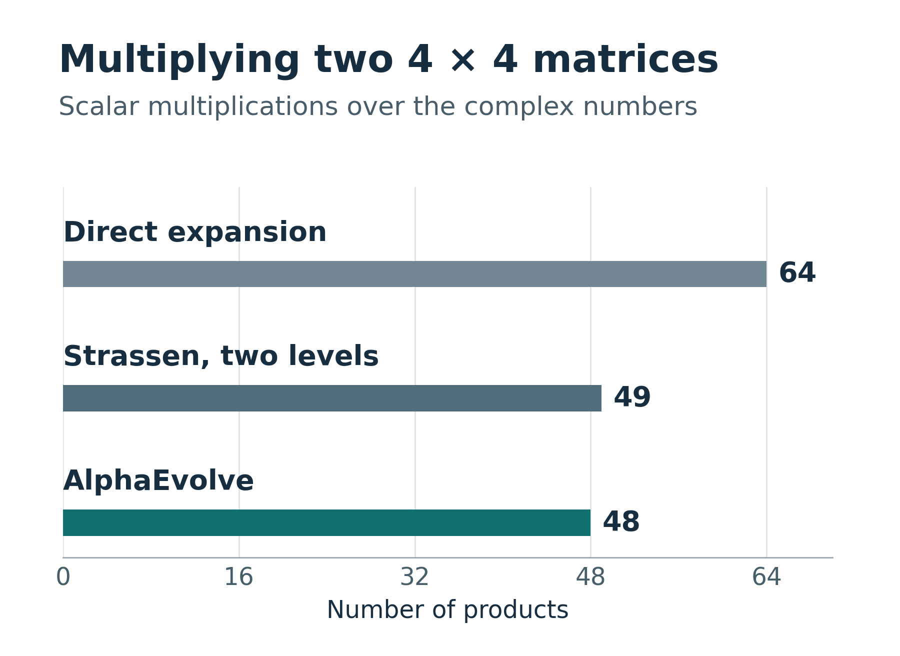
Work through the supplementary chart from the first entry. A 4×4 matrix product has 16 output entries, each a dot product of length four. Direct evaluation takes 16×4=64 scalar multiplications. Strassen’s method uses seven products at the 2×2 block level. Applying it twice gives 7×7=49. The discovered procedure uses 48 for the same 4×4 complex matrix product. Going from 49 to 48 saves one multiplication. Additions, memory transfers and elapsed time on particular hardware require separate measurements. AlphaEvolve, Table 2 · Complex arithmetic and the reported result
#Worked example 7. How does ShinkaEvolve score both prediction loss and expert imbalance?
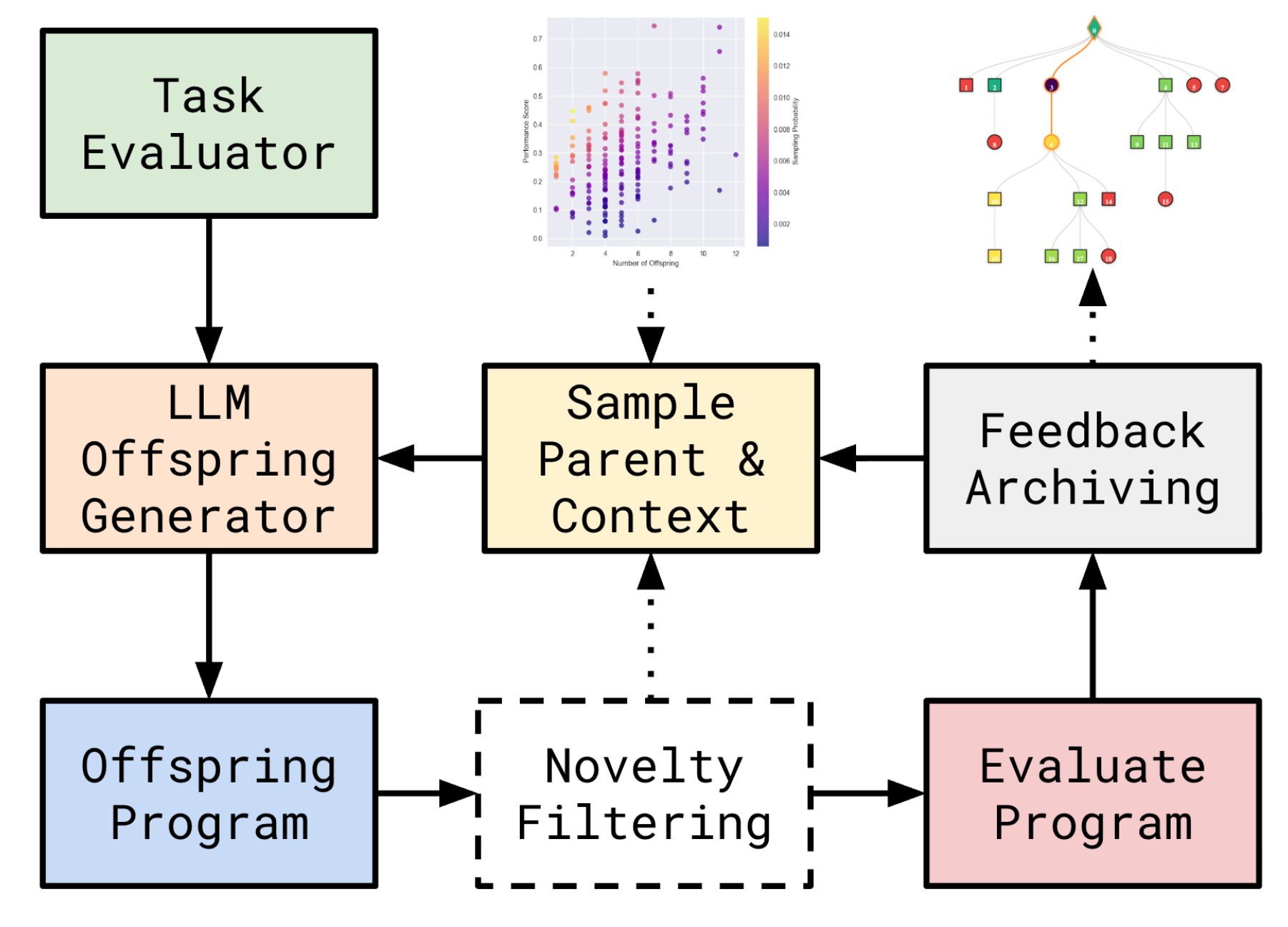
In a mixture of experts (MoE), a router chooses which experts process each token. In the September 2025 ShinkaEvolve paper, the code under evolution computed an auxiliary loss that discouraged unbalanced routing during training. The team evaluated candidates on a 556-million-parameter model with 64 experts, activating eight per token. Inner training added 0.01 times the candidate auxiliary loss to next-token cross-entropy (CE). Outer evaluation measured the trained model’s CE and its actual routing imbalance. Follow the arrow from evaluation back to the archive in the supplementary figure to locate this second comparison. ShinkaEvolve, §4.4
Work through Equations 4–5 in the appendix. For this example, use two experts and send each token to one expert. After training with candidate A, 60 of 100 tokens go to one expert and 40 to the other. The final CE is 2.00. For candidate B the counts are 52 and 48, and CE is 2.05. Uniform routing would give each expert a share of 0.5. Sum the absolute differences between each observed share fᵢ and that target, then divide by two. ShinkaEvolve, Appendix B.4, Equations 4–5
Higher scores win, so B leads by 0.03. It pays 0.05 in CE and gains 0.08 by reducing imbalance. The earlier 0.01 controls the candidate auxiliary loss during model training. Multiplying D by it during outer scoring would change the selection criterion. The actual search ran for 30 iterations because each pretraining run was expensive. Final CE was averaged over the last ten million tokens. Evaluation procedure and fitness equation
The θ′ on page 41, the staircase on page 44 and the proposed algorithm on page 45 record three different outputs. The first is a model’s weights, the second tracks the validation record across training runs, and the third is a procedure ready for another run. Page 46 turns to SEAL. When a model proposes material for its own training, what result should earn that proposal a good score? NTU Part II, page 46
Paper figure licenses. PostTrainBench and ShinkaEvolve