An inspection camera reads the digit 0 in a part number as the letter O. Someone adds “check for a zero first in a numeric field” to the reading instructions, and errors fall. So far, the inspection instructions have improved. Now suppose the next time a different error appears, the system also changes which failures it reads first and how it proposes a revision. That changes how edits are made. How could we tell which of the two improvements we are seeing?
Chapter 20 tested whether old skills survived a change to an agent’s harness, the code and instructions around its model. Pages 36–40 of Part II turn to the improver itself. Hyperagents gives us an agent and a candidate-selection rule to examine. Learning to Self-Evolve shows how researchers train a model to edit context. The camera and part numbers are worked examples. The paper figures and tables carry the experimental results.
Worked examples Matched editors · Math accuracy · Improvement in 50 iterations · Choosing a parent · Reading the three scores · Reward for an edit · Updating edit probability
Video guide by slide
| Part II page | Lecture video | What to listen for |
|---|---|---|
| 36 | 35:08 | How does the lecture move from a fixed editor to an agent that edits itself? |
| 37 | 35:16 | What does it mean for a revised harness to act as the next editor? |
| 38 | 35:48 | Who chooses the starting point for the next edit from a pool of candidates? |
| 39 | 36:33 | How did three parent-selection rules compare on training and test tasks? |
| 40 | 37:29 | What signal should train the model that proposes an edit? |
Each link opens the discussion of that topic. NTU lecture for May 22, 2026
#Part II, page 36 — What gets edited, and who does the editing?
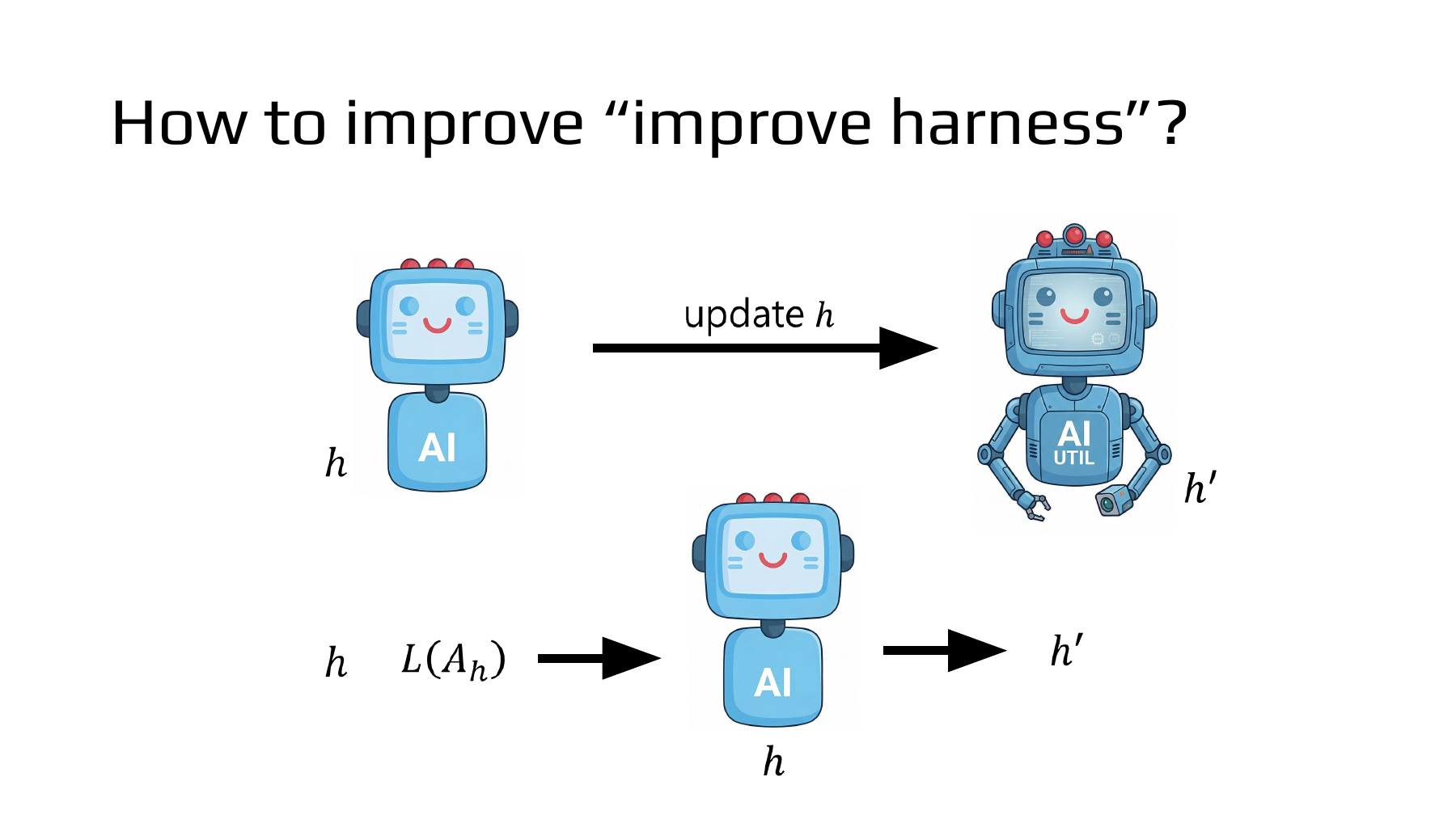
The top row, h → h′, shows the inspection agent’s harness changing to a new version. The bottom row uses h twice. The h on the left is the object to be edited. Beside it, L(Aₕ) is the loss incurred by the agent when it performs the task with that harness. The h beneath the central robot is the harness of the agent that reads this information and proposes an edit. The current agent can therefore edit its own harness. For that edit to change how the next generation improves itself, it must affect the part that proposes the next edit. NTU lecture, 35:08
#Worked example 1. Does changing one editing rule help two different inspectors?
Consider a tabletop camera that inspects parts. In this hypothetical experiment, inspector A sometimes fails on reflections from metal, while inspector B struggles with partly occluded edges. Give the original editing rule U₀ and its replacement U₁ the same parent inspector and the same failure records. Each rule gets one edit under the same model-call and token budget. For each parent, set aside 20 labeled images that the editors never see. Score the parent and both children on those same 20 images.
| Parent inspector | Correct before editing | After an edit by U₀ | After an edit by U₁ |
|---|---|---|---|
| A · metal reflections | 14/20 | 15/20 | 17/20 |
| B · occluded edges | 16/20 | 18/20 | 17/20 |
Let Δᵢ(U) be the accuracy gain produced by rule U on parent i, and nᵢ the number of correct predictions in the table. Editing A with U₁ adds three correct predictions, a 15-percentage-point gain. Editing B with U₁ adds one, a gain of 5 points.
Under the original rule U₀, A gained 5 points and B gained 10. Subtract the two rules’ gains within each parent, then take the mean, weighting each parent equally.
Changing the rule produced an average additional gain of 2.5 percentage points. For reflection-prone A, U₁ gained 10 points more than U₀. For edge inspector B, it gained 5 points less. Those differences disappear if we look only at the two final U₁ scores, both 17/20. Evidence that the editor also improves in a new inspection setting would require further parent inspectors and independently repeated edits.
#Supplementary lecture · How do we test the ability to adapt to a new task?
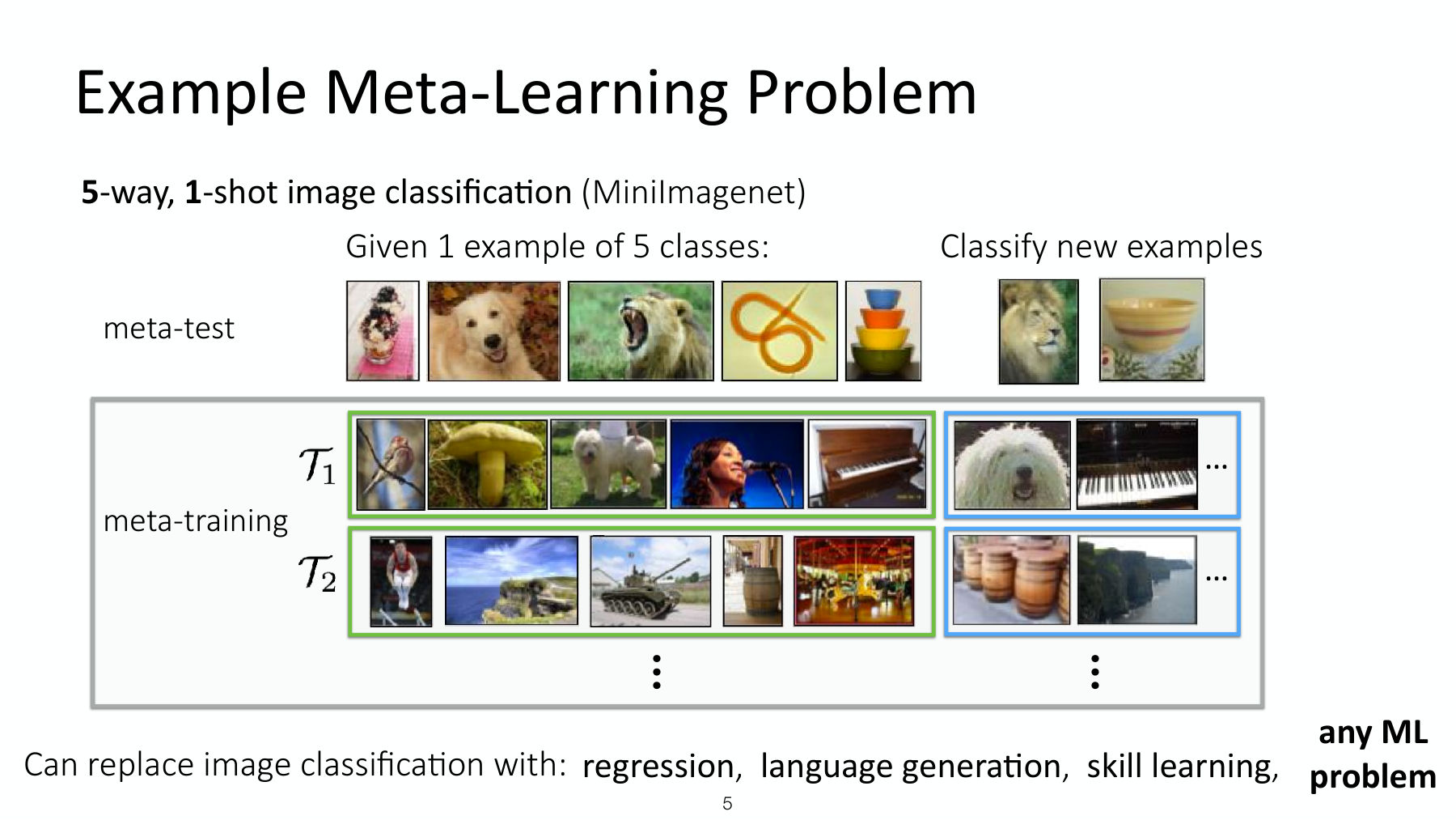
In Stanford CS330’s MiniImageNet diagram, one task is a five-class image classification problem. 5-way counts the classes in that task. 1-shot means that the learner sees one labeled image per class. Given those five images, it classifies other images from the same classes. At meta-test time, tasks are built from classes unseen during meta-training to check whether the adaptation procedure transfers. The connection to the two inspectors is in the evaluation design. Keep the evidence used for adaptation separate from the examples used to score the result, and vary the starting task. The Stanford example measures adaptation to new classes. The self-editing harness is the additional mechanism in the NTU example. Stanford CS330, Optimization-Based Meta-Learning, p. 5
#Part II, page 37 — The revised agent becomes the next editor
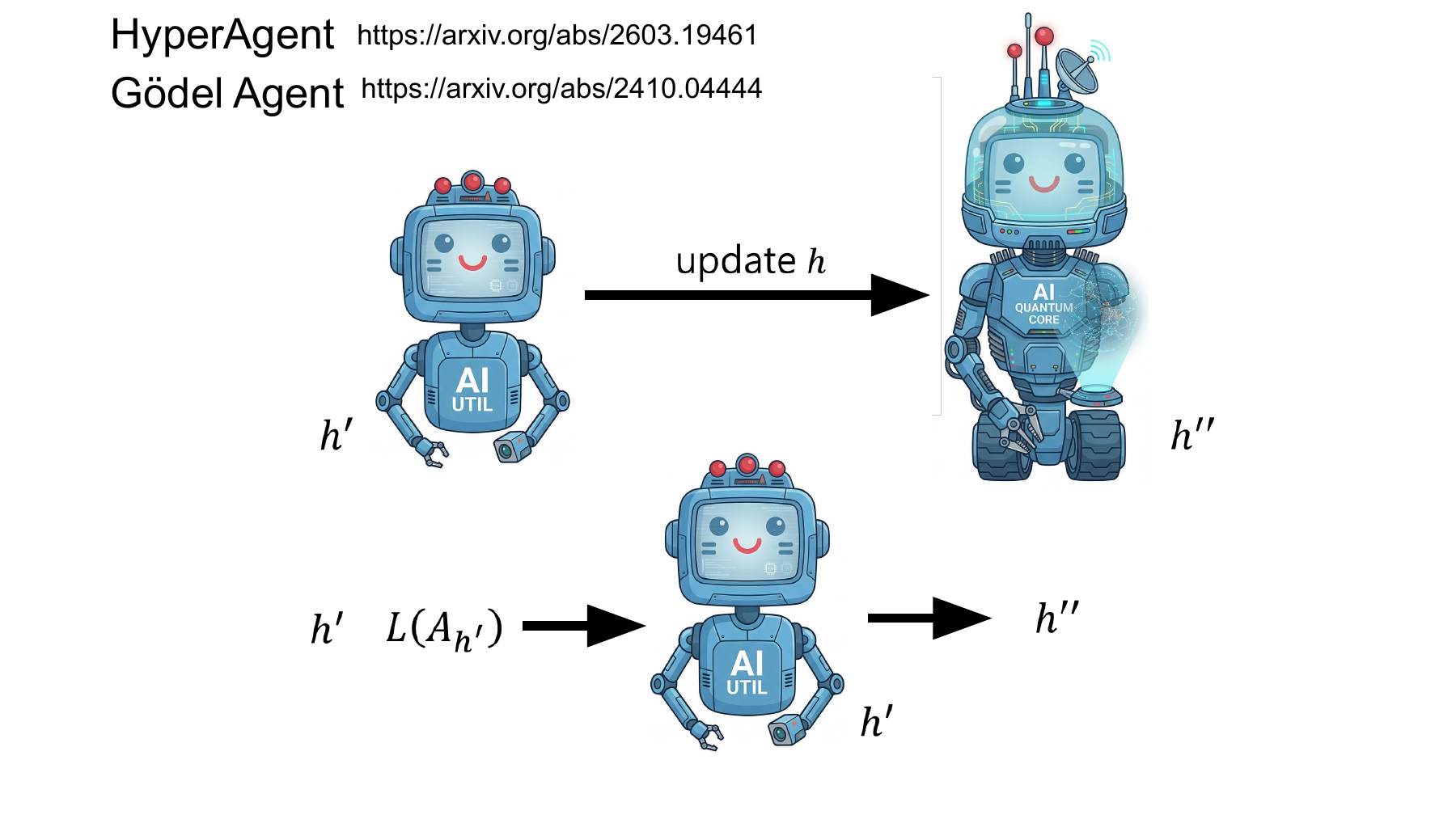
In the top row, h′ is a harness that has already been revised once. The arrow leads to its successor, h″. In the bottom row, h′ appears twice. On the left it labels what gets edited. On the robot in the middle it identifies who does the editing. That robot receives the current version and feedback from its execution, L(A_h′), and proposes the next version. Consider a math grader. Revising its marking rules can change the grade it assigns today. Revising how it selects errors to review during the next revision can also change which grader it produces tomorrow. We can test those capabilities separately. NTU slide 37
In Figure 1 of Zhang and colleagues’ Hyperagents, the task agent takes an input and performs the task. The meta agent proposes a new agent. Both live in one program, so a child can inherit both a method for solving a task and a method for generating successors. Assigning accurate grades to Olympiad solutions and improving the grader are separate abilities. The authors measured both the score of a grader and the improvement an editor could produce within a limited number of revisions. The figures here come from the March 2026 version available before the May NTU lecture. Hyperagents, Fig. 1 and §3
At three minutes in the ACL author presentation, one slide compares a hand-designed agent, automated design with a fixed editor, and a design that can modify its editor. Follow the returning arrow in the right-hand design. Then pause at 6:02 to see how the authors evaluated the resulting agent on individual tasks. ACL presentation, 3:00 · three designs · 6:02 · task results
#Worked example 2. What does a 10.8-point difference in math accuracy measure?
The other paper cited on the slide, Yin and colleagues’ Gödel Agent, allows changes to both the policy that performs a task and the procedure that improves the policy. Table 1 evaluates the resulting task-solving policy on MGSM, a multilingual collection of grade-school math word problems. The matched comparison uses Gödel-base, which is closed-book and uses GPT-3.5 to execute the final policy. The MGSM evaluation used 128 validation problems and 800 test problems. Meta Agent Search achieved 53.4% test accuracy and Gödel-base achieved 64.2%. Gödel Agent, Table 1 · Appendix B, evaluation protocol
The difference between the two accuracies is 10.8 percentage points. Relative to the 53.4% baseline, that is a 20.2% increase. Gödel-free scored 90.6% in the same table under different execution constraints, so it falls outside this comparison. The two matched scores tell us which resulting policy answered more MGSM problems correctly. Measuring the editor’s own ability to improve calls for observing the successors it produces on a new task.
#Worked example 3. Hold the editor fixed and measure its gain over 50 revisions
The Hyperagents authors transferred agents developed in paper review and robotics reward design to grading Olympiad-level math solutions. The grader receives a problem, a candidate solution, reference solutions, and grading guidelines. It predicts one of the expert grades 0, 1, 6, or 7. Accuracy is the fraction of solutions whose predicted grade matches the expert’s grade, with 100 examples in each of the training, validation, and test splits. Could the transferred meta agent, held fixed, produce a better task agent in this new domain? Hyperagents, §5.2 · Appendix C.4, grading data
Generate candidates for up to k revisions, then select a candidate by validation accuracy. The difference between that candidate’s test accuracy and the starting agent’s test accuracy is improvement@k. Here A₀ is the starting grader and Aᵢ is the ith candidate.
This is the reported median across five runs. The transferred agent began at zero on the new task. The candidates produced by its meta agent, selected on validation data, reached a median test score of 0.630 (95% bootstrap confidence interval for the gain, 0.540–0.630). With the same 50-revision budget, fixing the original, inexperienced meta agent instead yielded a median gain of 0.000. Fifty counts revisions. One hundred counts test solutions. The 0.630 measures agreement with expert grades. It does not count Olympiad problems solved by the agent. Hyperagents, Fig. 3 and accompanying text · Transfer results
#Part II, page 38 — Which parent to revisit can change too
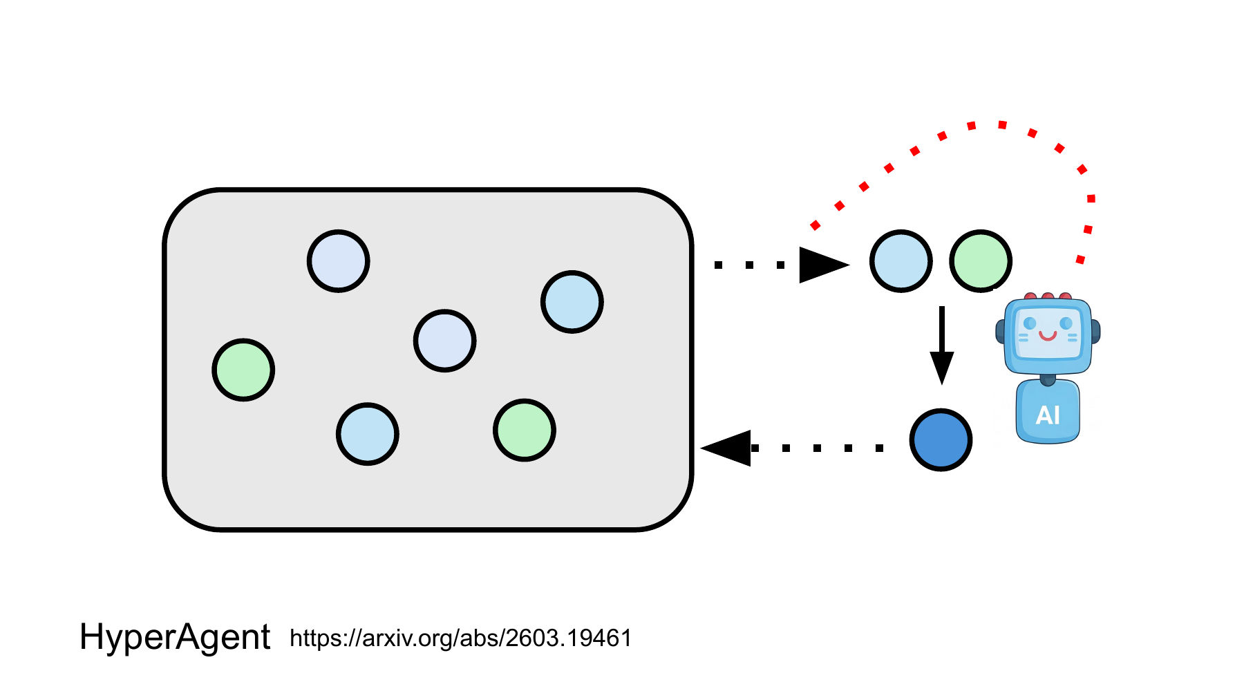
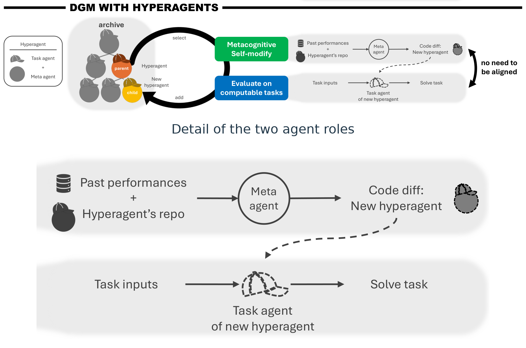
The gray box is an archive of past candidates. Follow the upper dotted arrow out of the archive to the candidates on the right, where a new candidate is produced. The lower dotted arrow returns it to the archive. The red dotted arc draws attention to a separate decision upstream. Which past version will serve as the starting point for the next revision? Page 37 considered changing how an editor works. Here the rule for choosing the parent it edits can change as well. The circles distinguish versions. The slide gives no score or dataset legend for their colors. NTU slide 38
The paper separates these choices experimentally. The main experiments fixed a handcrafted parent-selection rule that accounts for performance and how many children a candidate already has. This lets the authors study changes to the editor separately. In the additional experiment in Appendix E.5, the system starts with random selection and may revise the selection rule itself. Across runs the authors observed variants of upper confidence bound (UCB) selection, which combine a performance score with an exploration bonus for less-tested candidates. Hyperagents, §3 · Appendix E.5, parent selection
#Worked example 4. Why revisit the parent with the lower score?
Suppose we are improving a grader. Parent A has a normalized evaluation score of 0.82 and has already produced 15 children. Parent B has a score of 0.70 and has produced three. We will plug illustrative values into the form of exploration bonus observed in the appendix. Let N be the total number of children, nᵢ the number from parent i, sᵢ its score, and c the weight on exploration. In this example we make one choice by taking the parent with the higher selection score U.
A leads by 0.12 on the evaluation score alone. B’s exploration bonus is about 0.343, compared with about 0.172 for A. Since the difference exceeds 0.12, the rule with c=0.4 chooses B. Lower c to 0.2 and A scores about 0.906 against B’s 0.872, reversing the choice. B’s 1.043 can exceed one because it ranks candidates. It is neither a predicted accuracy nor a probability that B’s child will succeed. Page 39 compares whether changing how parents are prioritized also changes final test performance. Hyperagents, Appendix E.5
#Part II, page 39 — Does letting agents choose their own parents produce better agents?
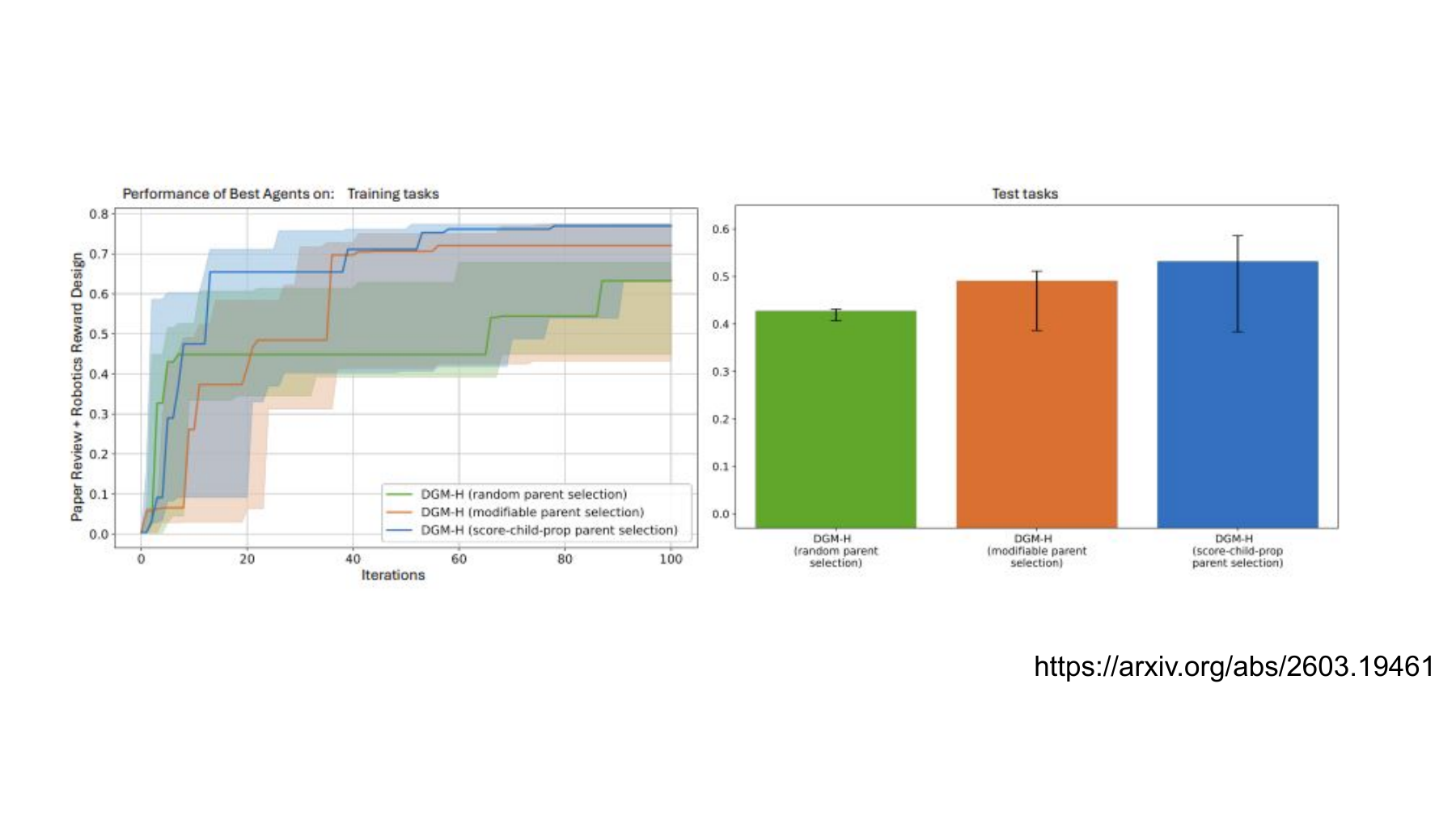
The red dotted arrow on page 38 suggests an experiment. Which agent emerges if the system can change how it chooses a starting point for the next edit? All three conditions generate and evaluate candidates. They differ in how they select the next parent. Green selects at random throughout. Orange starts with random selection and can revise the selection rule. Blue keeps the researchers’ rule, which accounts for a candidate’s score and the number of its children that compiled successfully. The authors ran each condition five times. NTU lecture, 36:33 · Hyperagents, version available at the time of the lecture, Appendix E.5
Read the left panel first. The horizontal axis counts iterations. The vertical axis averages scores in two domains, paper review and reward design for simulated robots. Each line tracks the best candidate found so far on training tasks. A low-scoring new candidate leaves the previous record intact. The right panel evaluates the best agents discovered by each method on held-out test tasks. The last point on a line and the corresponding bar come from different problems.
#Worked example 5. How large is the gain in the orange bar, and how uncertain is it?
| Parent selection | Reported test score | Reported confidence interval |
|---|---|---|
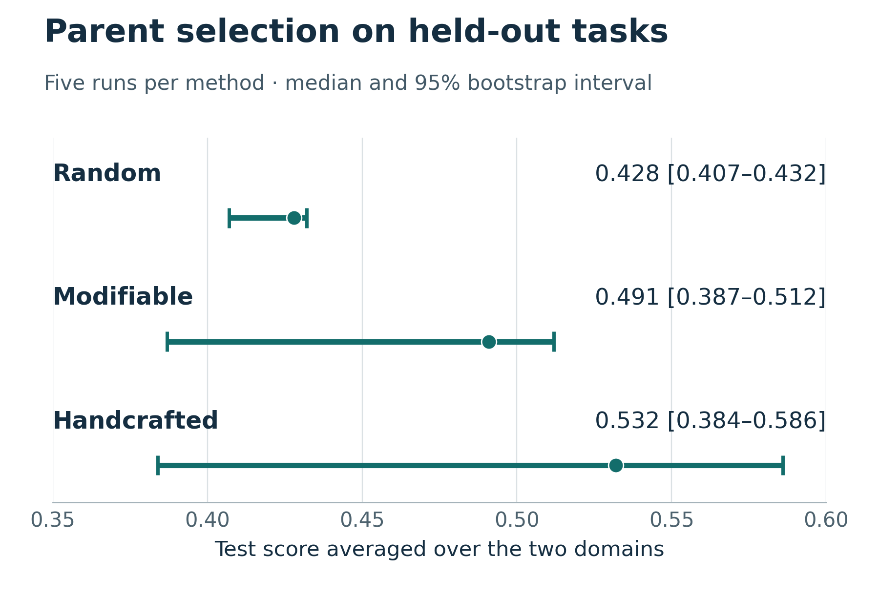
| Fixed random selection | 0.428 | 0.407–0.432 |
| Start at random and allow edits to the selection rule | 0.491 | 0.387–0.512 |
| Fixed rule devised by the researchers | 0.532 | 0.384–0.586 |
The table combines two kinds of aggregation. The score for one run is the mean of its two domain scores. The representative score for each method is the median across runs. The authors obtained 95% bootstrap confidence intervals by resampling the five runs 1,000 times. The following subtraction compares the reported medians. Statistical protocol · Figure 11 and reported scores
The initial agent scored 0.030. Measured from that starting point, the median in the orange condition rose by 0.461. To ask how much of that gain is associated with permission to edit the selection rule, compare it with the condition that keeps improving candidates while continuing to choose their parents at random.
The observed difference is 0.063 score units. Because the score combines both domains, it cannot tell us how much the robot’s success rate changed. Across five runs, the authors found no statistically significant difference between conditions (p > 0.05). The blue bar had the largest median in this experiment. The five runs leave uncertainty about the ranking in future experiments.
#Part II, page 40 — What reward should an editor receive for a good revision?
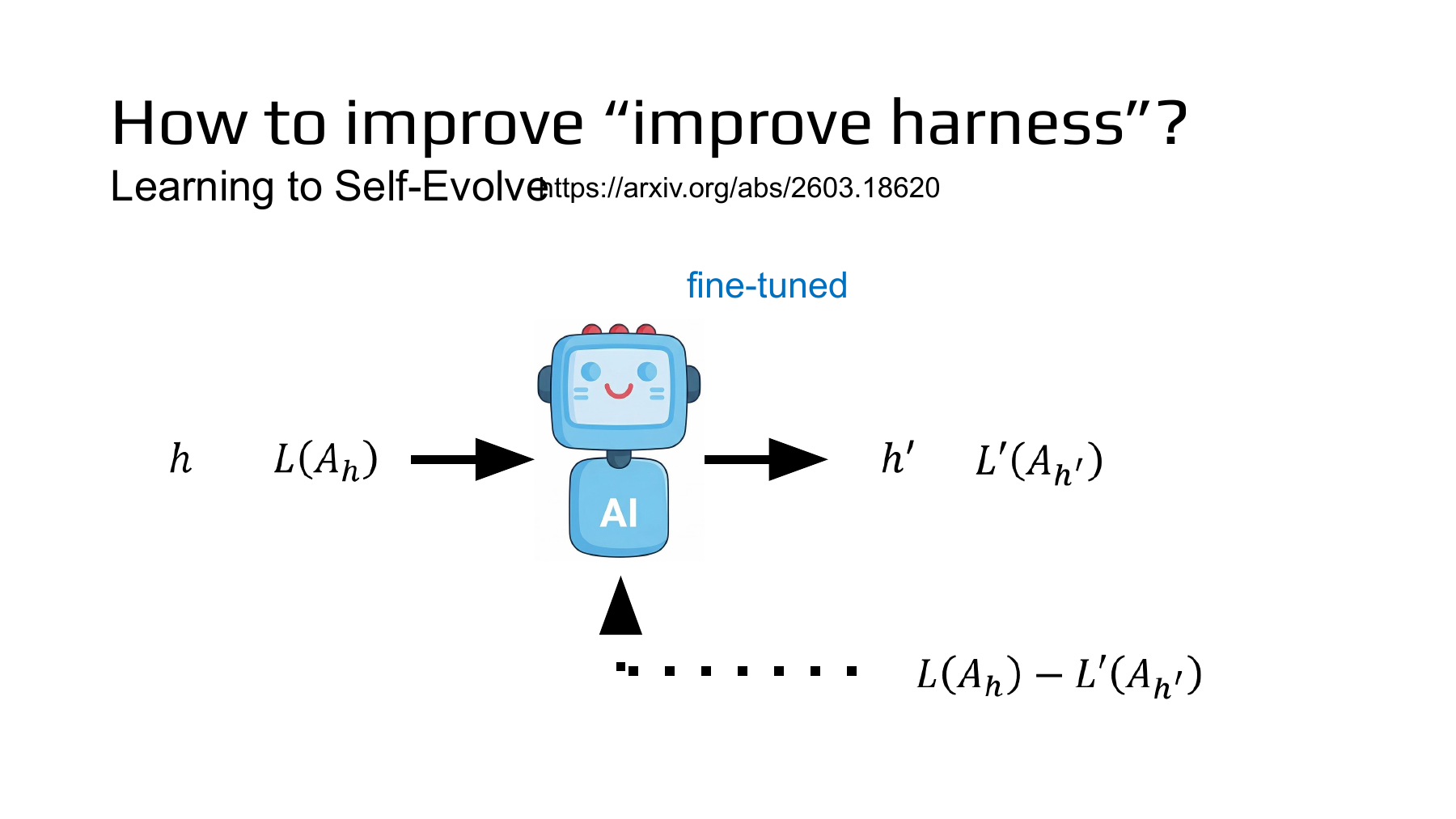
Trace the two arrows into the blue robot. From the left come the current harness h and its recorded performance. The robot proposes an edited harness h′. The dotted line then feeds the original loss minus the post-edit loss back to the editor. Page 38 examined changes to a selection rule. Here, “fine-tuned” labels the model that proposes revised instructions. NTU lecture, 37:29 · Lee compares the two scores at 38:20
In Chen and colleagues’ Learning to Self-Evolve (LSE), an action policy solves problems under a given context. An editing policy reads that context and feedback from previous attempts and revises the instruction field. Training updates the editor’s weights. At test time, the trained editor proposes a series of contexts, while the action policy’s weights stay fixed. In the figure, follow the multi-round search on the left and the single-step training signal on the right. LSE, Figure 1 · Sections 3.1–3.2
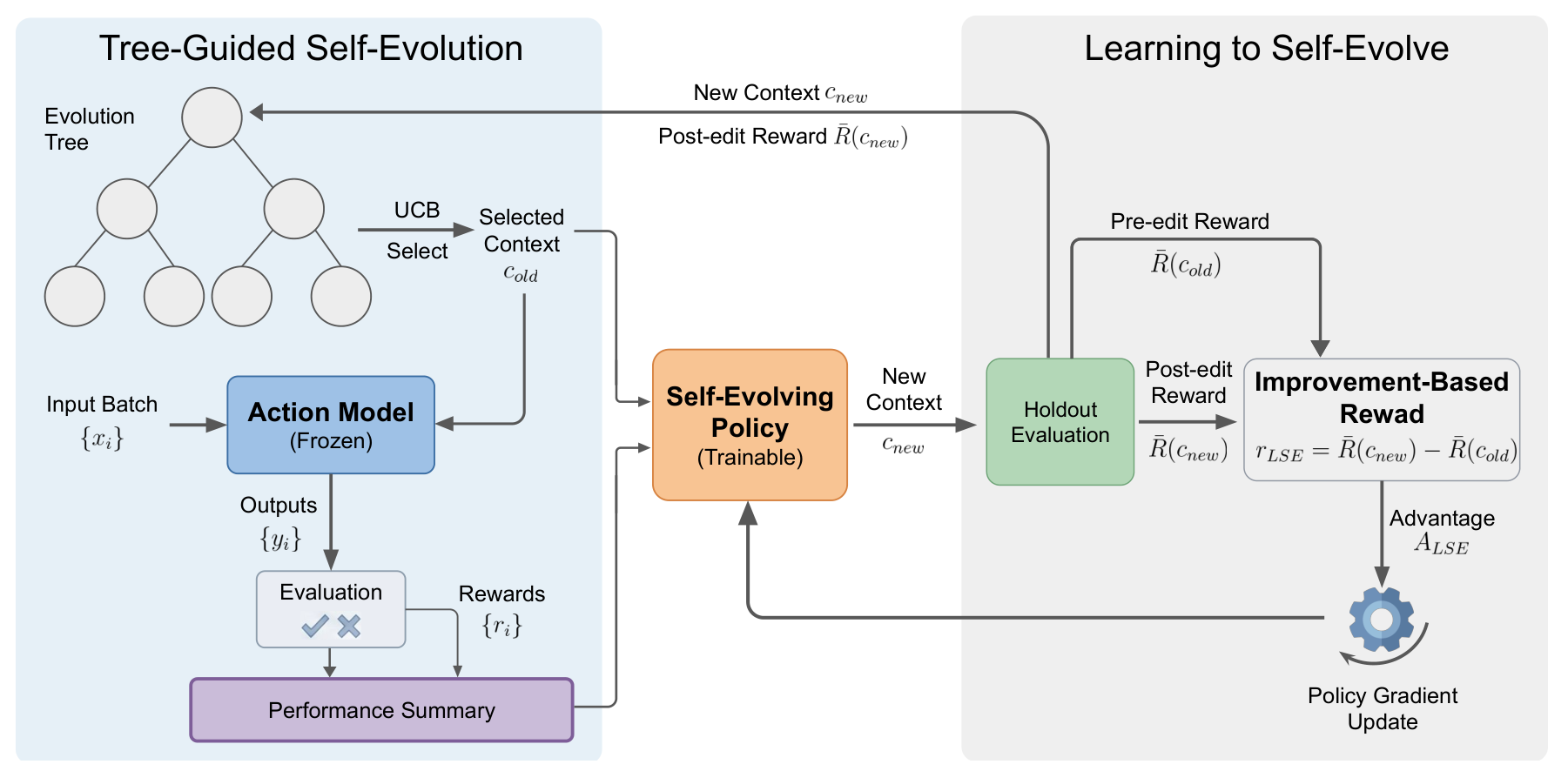
#Worked example 6. Why can a high final score still give the editor a negative reward?
Consider a hypothetical edit to an instruction for reading part numbers in inspection images. Within each row, score both versions on the same 20 images, awarding one point for each correct part number. Starting instruction A goes from 16 correct to 15. Starting instruction B goes from 9 to 13.
| Starting instruction | Accuracy before editing | Accuracy after editing | Gain from this edit |
|---|---|---|---|
| A | 16/20 = 0.80 | 15/20 = 0.75 | −0.05 |
| B | 9/20 = 0.45 | 13/20 = 0.65 | +0.20 |
A delivers the higher final score. The ranking changes when we ask what the edit accomplished. The net change in correct predictions is a loss of one for A and a gain of four for B. Equation 7 of the paper denotes the mean reward under context c by R̄(c) and subtracts the pre-edit reward from the post-edit reward. The slide uses loss, where smaller values are better, so the order is reversed. If loss is the error rate, the two expressions agree exactly.
If we score an edit on easier images than its starting instruction, the measured difference also picks up the change in difficulty. The paper compares contexts on a fixed holdout set separate from the batches that supply feedback each round. Repeatedly using that holdout to select candidates also gives its score a different interpretation from a one-time evaluation on fresh data. LSE, Equation 4 · Equation 7 and evaluation procedure
#Worked example 7. How does that reward change the chance of proposing the same edit again?
Suppose the policy can propose either of two edits, A and B, from the same starting context. This calculation is independent of the preceding table. A raises accuracy by 0.15 and B lowers it by 0.05. With probability p of proposing A and probability 1−p of proposing B, the expected gain J for one edit is
Let z be the difference between the policy’s two logits, its preference scores before normalization, and compute p with a sigmoid. When z is zero, the two edits are equally likely. The gradient at that point is 0.05. Take one step with a learning rate of 0.4 in the direction that increases expected gain.
The chance of proposing A rose from 50% to about 50.5%. That 50.5% measures the probability of choosing a particular edit. Part-number recognition accuracy measures the performance of the resulting instruction. In Equations 9–10, the authors sample an actual text edit and weight the gradient of its log probability by the measured improvement. With just two possible edits in our example, we could differentiate the expected gain directly. LSE, Equations 9–10
#Supplementary paper · Which model did what to earn 67.3%?
In BIRD, the task is to translate natural-language questions into SQL. Accuracy is measured by executing the resulting queries. Qwen3-4B-Instruct writes the SQL in every row of Table 1. The methods differ in how they produce the instructions. Across the five database domains, LSE scored 72.0, 68.5, 72.0, 59.8 and 64.0%. With equal weight per domain, the mean is 67.26%, or 67.3% after rounding. The starting instructions scored 57.2%, the Qwen editor without specific training for editing scored 62.2%, and the GPT-5 editor scored 65.2%. With the same action model, the LSE-trained editor gained 10.1, 5.1 and 2.1 percentage points over those baselines, respectively. Within each domain, the authors averaged performance over eight generations on a fixed holdout of 50 problems and reported the best holdout performance reached in 25 rounds of evolution. LSE, Table 1 · Section 4.2, main results · Appendix A, evaluation procedure
In Part 20, we repeated the same task before and after an edit to see whether the agent retained a skill. Here we need one more record. Which editor produced the gain, from which starting point, and on which evaluation problems? Recording all three lets us test the quality of a harness and the ability to improve a harness separately. On page 41, the lecture turns to updating model parameters. NTU Part II, p. 41
The Hyperagents and Learning to Self-Evolve figures are credited in their captions. License for these paper figures